CSE 431/531 · Module 08 · Week 6
Coping with NP-Completeness
Backtracking, branch and bound, approximation algorithms with guarantees, and local search heuristics.
Companion reading: Dasgupta, Papadimitriou & Vazirani, Algorithms, chapter 9, “Coping with NP-completeness”
By the end of this module you can
- Design a backtracking algorithm from three parts (a test, a rule for choosing a subproblem, and a rule for expanding it), and explain why branching on a smallest clause helps for SAT.
- Turn backtracking into branch and bound for a minimization problem, and prove that the minimum-spanning-tree bound for the traveling salesman problem is a valid lower bound.
- Define the approximation ratio, and prove factor-2 guarantees for vertex cover, k-clustering, and metric TSP by comparing each algorithm with a lower bound on the optimum.
- Prove that the general traveling salesman problem has no polynomial-time approximation algorithm with a constant ratio unless P = NP.
- Build the rounding scheme for knapsack and derive its \((1-\epsilon)\) guarantee and \(O(n^3/\epsilon)\) running time.
- Design a local search by choosing a neighborhood, explain the tradeoff between neighborhood size and solution quality, and use random restarts and simulated annealing to escape poor local optima.
- Place an NP-hard optimization problem in the approximability hierarchy and pick a sensible way to attack it.
Contents
- Before giving up on exactness
- Intelligent exhaustive search
- Approximation algorithms
- Local search heuristics
- Summary
- Exercises
- Going further
Module 07 ended with a long list of problems — SAT, 3SAT, independent set, vertex cover, clique, the traveling salesman problem, Rudrata cycle, integer programming — that are all NP-complete. None of them has a polynomial-time algorithm unless P = NP, and most computer scientists believe P ≠ NP. So what do you do on Monday morning, when the problem on your desk turns out to be one of them?
Proving NP-completeness is useful: it tells you to stop looking for a fast exact algorithm that works on every input. But the problem does not go away. This module collects the standard ways to cope. We can give up a little on running time and search the exponential space cleverly (backtracking and branch and bound). We can give up a little on quality and settle for an answer that is provably close to optimal (approximation algorithms). Or we can give up on guarantees altogether and use methods that work well in practice (local search and its relatives). Each part ends with code you can run and measure against a brute-force optimum on small inputs.
This is the last module of the course, so the summary closes with a short look back over the whole term.
Before giving up on exactness
An NP-completeness proof shows that the general problem is hard. The hard instances it builds are usually strange — graphs assembled from gadgets, formulas with carefully planted clauses — and may look nothing like the instances you care about. So the first question is whether your inputs belong to an easier special case.
- SAT is NP-complete, but Horn formulas can be tested for satisfiability in polynomial time by the greedy algorithm of module 05, and formulas with at most two literals per clause (2SAT) can be solved in linear time with strongly connected components (module 03; DPV exercise 3.28).
- Independent set is NP-complete on general graphs, but on trees a dynamic program over the subtrees finds a largest independent set in linear time (module 06, DPV section 6.7).
- Knapsack is NP-complete, but the dynamic program of module 06 runs in \(O(nW)\) time, which is fast whenever the capacity \(W\) is small.
This does not always rescue us. 3SAT is itself a special case of SAT, and it is still NP-complete; independent set stays NP-complete even on planar graphs. And often the instances that arise in an application have no clean description at all. Then we turn to one of three strategies, which trade away different things:
| Strategy | Running time | Quality of the answer |
|---|---|---|
| Intelligent exhaustive search (backtracking, branch and bound) | exponential in the worst case, often fast in practice | optimal |
| Approximation algorithms | polynomial, guaranteed | within a proven factor of optimal |
| Heuristics (local search, simulated annealing) | usually fast, rarely guaranteed | no guarantee, often very good |
Intelligent exhaustive search
A brute-force search tries every candidate solution: all \(2^n\) truth assignments, all \((n-1)!\) tours. The two methods in this section search the same space, but they organize it as a tree of partial solutions and throw away whole subtrees as soon as they can tell that nothing useful lies below. In the worst case they still take exponential time. In practice, with good rules for pruning, they often explore a tiny fraction of the space.
Backtracking
The observation behind backtracking is that you can often reject a solution after looking at only a small part of it. Suppose a SAT formula contains the clause \((\overline{x_2} \lor x_3)\). Every assignment with \(x_2 = 1\) and \(x_3 = 0\) falsifies that clause, so as soon as we have set those two variables that way, we can discard the entire family of \(2^{n-2}\) completions — a quarter of the search space — without looking at any of them.
To make this systematic, grow a tree of partial assignments. Each node fixes some of the variables. Plugging those values into the formula leaves a smaller formula, the residual formula: clauses that already contain a true literal are satisfied and disappear, and false literals are deleted from the clauses that remain. So every node of the tree is itself a SAT instance, a subproblem, on fewer variables. A clause from which every literal has been deleted is the empty clause, written \(()\); it can never be satisfied, so a subproblem that contains it is dead.
In code, a formula in conjunctive normal form is a list of clauses, and a clause is a tuple of nonzero integers: \(i\) stands for the literal \(x_i\) and \(-i\) for \(\overline{x_i}\) (the convention used by SAT solvers’ input files).
import heapq, itertools, math, random
from collections import namedtuple

def assign(formula, lit):
    """Residual formula after making literal lit true."""
    residual = []
    for clause in formula:
        if lit in clause:                   # clause satisfied: drop it
            continue
        # -lit is now false: delete it from the clause
        residual.append(tuple(l for l in clause if l != -lit))
    return residual

phi = [(1, 2), (-1, 3), (-2, 3), (-3, 4), (-3, -4), (1, -2, 4)]
print(assign(phi, -1))                 # x1 = 0
print(assign(assign(phi, -1), -2))     # x1 = 0, x2 = 0
[(2,), (-2, 3), (-3, 4), (-3, -4), (-2, 4)]
[(), (-3, 4), (-3, -4)]
The formula phi is
Setting \(x_1 = 0\) leaves a one-literal clause \((x_2)\); setting \(x_2 = 0\) as well produces the empty clause, so that branch is finished.
The backtracking template
A backtracking algorithm relies on a fast test that examines a subproblem and returns one of three verdicts:
- failure: the subproblem certainly has no solution;
- success: a solution has been found;
- uncertain: we cannot tell yet.
For SAT the test is immediate: an empty clause means failure, a formula with no clauses left means success, and anything else is uncertain. Around the test, the algorithm keeps a set of active subproblems and repeats: choose an active subproblem, expand it into smaller subproblems, and test each one. Successes end the search, failures are discarded, and uncertain subproblems become active. If the active set runs dry, there is no solution.
def backtrack(root, expand, test, priority):
    """Generic backtracking search.
    expand(P): list of smaller subproblems.
    test(P):   "success", "failure", or "uncertain".
    choose:    the active subproblem with the smallest priority(P).
    Returns (solution subproblem or None, number of subproblems tested)."""
    tested = 1
    outcome = test(root)
    if outcome != "uncertain":
        return (root if outcome == "success" else None), tested
    tick = itertools.count()     # tie-breaker: heapq never compares subproblems
    active = [(priority(root), next(tick), root)]
    while active:
        _, _, P = heapq.heappop(active)                   # choose
        for Q in expand(P):                               # expand
            tested += 1
            outcome = test(Q)
            if outcome == "success":
                return Q, tested
            if outcome == "uncertain":
                heapq.heappush(active, (priority(Q), next(tick), Q))
            # on "failure", Q is simply dropped: this is the pruning
    return None, tested
The two design decisions are which subproblem to choose and which variable to branch on. Pruning happens only when an empty clause appears, and a clause becomes empty fastest when it is short. That suggests the rule: choose the active subproblem with the smallest clause, and branch on a variable of that clause. If that clause has a single literal, one of the two branches makes it empty and dies at once, so the tree does not really branch at all. When several subproblems tie, take the deepest one, since it has the most variables set and may be closest to a satisfying assignment.
SatNode = namedtuple("SatNode", "formula assignment depth")

def sat_test(P):
    if not P.formula:
        return "success"
    if any(len(c) == 0 for c in P.formula):
        return "failure"
    return "uncertain"

def smallest_clause_first(P):
    """Priority: shortest clause first; among ties, deepest node first."""
    return (min(len(c) for c in P.formula), -P.depth)

def expand_on_smallest_clause(P):
    """Branch on a variable of a shortest clause: x = 0, then x = 1."""
    x = abs(min(P.formula, key=len)[0])
    return [SatNode(assign(P.formula, lit), {**P.assignment, x: lit > 0},
                    P.depth + 1)
            for lit in (-x, x)]

def backtrack_sat(formula):
    root = SatNode(formula, {}, 0)
    node, tested = backtrack(root, expand_on_smallest_clause,
                             sat_test, smallest_clause_first)
    return (node.assignment if node else None), tested

backtrack_sat(phi)
(None, 13)
The answer None means phi is unsatisfiable, and the search tested 13 subproblems to prove it. You can check the verdict by hand: the first three clauses force \(x_3 = 1\) (if \(x_1 = 1\) the second clause needs \(x_3\); if \(x_1 = 0\) the first clause needs \(x_2\), and then the third needs \(x_3\)), and then clauses four and five demand both \(x_4\) and \(\overline{x_4}\). The figure shows the search tree.
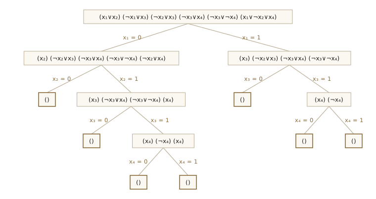
phi (¬ marks a negated literal), branching on a variable of a shortest clause. Each node shows the residual formula of its partial assignment; the brass () leaves contain the empty clause and are pruned (their other clauses are omitted). Once a one-literal clause appears, every branching step kills one of its two children immediately.A satisfying assignment that backtracking returns may leave some variables unset (any value works for them). A brute-force search for comparison, and a check:
def satisfies(formula, assignment):
    """Does every clause have a true literal? (Unset variables count as 0.)"""
    return all(any(assignment.get(abs(l), False) == (l > 0) for l in clause)
               for clause in formula)

def brute_force_sat(formula, n):
    """Try all 2^n assignments; return (assignment or None, number tried)."""
    tried = 0
    for bits in itertools.product([False, True], repeat=n):
        tried += 1
        a = dict(zip(range(1, n + 1), bits))
        if satisfies(formula, a):
            return a, tried
    return None, tried

def random_3sat(n, m, rng):
    """m random clauses, each on 3 distinct variables with random signs."""
    clauses = []
    for _ in range(m):
        variables = rng.sample(range(1, n + 1), 3)
        signs = [rng.choice([1, -1]) for _ in variables]
        clauses.append(tuple(s * v for s, v in zip(signs, variables)))
    return clauses

rng = random.Random(8)
sat_count = 0
for _ in range(100):
    F = random_3sat(10, 43, rng)
    a, _ = backtrack_sat(F)
    b, _ = brute_force_sat(F, 10)
    assert (a is None) == (b is None)      # same verdict
    assert a is None or satisfies(F, a)    # and a real solution if there is one
    sat_count += a is not None
print(f"100 random formulas (n = 10, m = 43): verdicts agree; "
      f"{sat_count} satisfiable")
100 random formulas (n = 10, m = 43): verdicts agree; 84 satisfiable
Now the point of the method: how much of the space does it explore? Random 3SAT formulas with about \(4.26n\) clauses are, experimentally, the hardest kind for backtracking (with many fewer clauses almost all are satisfiable and easy; with many more, almost all are quickly refuted), so that is what we test on.
rng = random.Random(1)
print("   n     m   satisfiable   subproblems tested      2^n")
for n in [20, 40, 60]:
    m = round(4.26 * n)
    for _ in range(3):
        F = random_3sat(n, m, rng)
        a, tested = backtrack_sat(F)
        print(f"{n:4d} {m:5d}   {str(a is not None):>11}   {tested:18,d}"
              f"   {2**n:.1e}")
   n     m   satisfiable   subproblems tested      2^n
  20    85          True                   89   1.0e+06
  20    85          True                   57   1.0e+06
  20    85         False                  207   1.0e+06
  40   170         False                2,003   1.1e+12
  40   170         False                1,481   1.1e+12
  40   170          True                  571   1.1e+12
  60   256         False                9,751   1.2e+18
  60   256          True               12,013   1.2e+18
  60   256         False                7,871   1.2e+18
The number of subproblems grows with \(n\), but it is a vanishing fraction of \(2^n\): at \(n = 60\), at most 12,013 subproblems stand in for about \(10^{18}\) assignments. Unsatisfiable formulas have to be refuted completely, so the search cannot stop early on them; satisfiable ones end as soon as a solution appears, which may still take a while. How much of that is due to the smallest-clause rule? Swap in a naive rule — always branch on the lowest-numbered remaining variable, deepest node first — and keep everything else the same:
def expand_on_lowest_variable(P):
    x = min(abs(l) for c in P.formula for l in c)
    return [SatNode(assign(P.formula, lit), {**P.assignment, x: lit > 0},
                    P.depth + 1)
            for lit in (-x, x)]

rng = random.Random(1)
print("average subproblems tested over 5 formulas")
print("   n   smallest clause   lowest variable")
for n in [15, 20, 25]:
    m = round(4.26 * n)
    totals = [0, 0]
    for _ in range(5):
        F = random_3sat(n, m, rng)
        totals[0] += backtrack(SatNode(F, {}, 0), expand_on_smallest_clause,
                               sat_test, smallest_clause_first)[1]
        totals[1] += backtrack(SatNode(F, {}, 0), expand_on_lowest_variable,
                               sat_test, lambda P: -P.depth)[1]
    print(f"{n:4d}   {totals[0] / 5:15,.0f}   {totals[1] / 5:15,.0f}")
average subproblems tested over 5 formulas
   n   smallest clause   lowest variable
  15                69               715
  20               128             3,994
  25               198            11,467
The naive rule tests far more subproblems, and the gap widens with \(n\). The smallest-clause rule wins because it keeps following one-literal clauses: once a clause is down to one literal, its value is forced, and setting it can shorten other clauses to one literal in turn. (SAT solvers call this unit propagation.) Branching decisions are made only when nothing is forced.
Note. Good choices for test, choose, and expand make backtracking a serious algorithm, not a stopgap. Backtracking with unit propagation, which the smallest-clause rule carries out automatically, is the heart of the Davis–Putnam–Logemann–Loveland (DPLL) procedure, the ancestor of most practical SAT solvers. On 2SAT formulas the smallest-clause rule even runs in polynomial time (exercise 1).
Branch and bound
Backtracking answers a yes-or-no question. Branch and bound adapts it to optimization. Take a minimization problem. Again each node of the search tree is a partial solution, standing for the subproblem “what is the cheapest way to complete this?”. A subproblem can be discarded when we are sure that every completion costs at least as much as the best complete solution found so far. We cannot afford to compute a subproblem’s exact cost — that is the whole problem — so instead we compute a quick lower bound on it. The template:
- Keep a set of active partial solutions, starting with the empty one, and
best_so_far\(= \infty\). - Repeatedly choose an active partial solution and expand it into its extensions.
- A complete extension updates
best_so_farif it is cheaper. An incomplete extension stays active only if its lower bound is belowbest_so_far; otherwise it is pruned. - When no active partial solutions remain,
best_so_faris optimal.
Correctness needs only one thing: the bound must never exceed the true cost of the best completion. Then a pruned subproblem cannot contain a solution better than one we already have. The quality of the bound decides the speed: the closer it is to the true cost, the earlier subproblems get pruned.
Branch and bound for the traveling salesman problem
In the traveling salesman problem (TSP) we are given \(n\) cities with distances \(d_{uv} > 0\) and want a tour, a cycle that visits every city exactly once, of minimum total length. Fix a starting city \(a\). A partial solution is a path from \(a\) to some city \(b\) through a set \(S\) of cities (including \(a\) and \(b\)); we write it \([a, S, b]\). Its subproblem is to find the cheapest way back: a path from \(b\) to \(a\) through all the cities in \(V - S\). The root is \([a, \{a\}, a]\), and expanding \([a, S, b]\) means adding one more edge \((b, x)\) for each \(x \in V - S\).
Lemma. Let \(R = V - S\) be nonempty. Every completion of \([a, S, b]\) costs at least the sum of (1) the lightest edge from \(a\) to \(R\), (2) the lightest edge from \(b\) to \(R\), and (3) the weight of a minimum spanning tree of \(R\).
Proof. A completion is a path \(b \to r_1 \to r_2 \to \dots \to r_k \to a\) that lists the cities of \(R\) in some order. Its first edge \((b, r_1)\) goes from \(b\) to \(R\), so it is at least the lightest such edge; similarly its last edge \((r_k, a)\) is at least the lightest edge from \(a\) to \(R\). The edges in between form a path through all of \(R\), which is a spanning tree of \(R\), so they weigh at least the minimum spanning tree. The three parts use disjoint edges, so the costs add. \(\square\)
Adding the cost of the path so far gives a lower bound on every full tour that extends \([a, S, b]\). The bound holds for any positive distances; it does not need the triangle inequality.
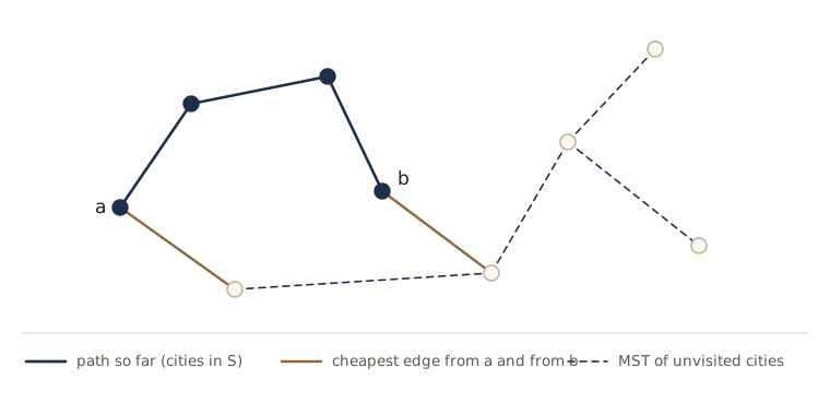
The minimum spanning tree comes from Prim’s algorithm (module 05). Here the graph is complete, so we use the version with a plain array of distances instead of a heap: each of the \(k\) rounds scans the remaining vertices, for \(O(k^2)\) time in all, which beats the heap version’s \(O(k^2 \log k)\) on a dense graph. Cities are points in the plane with Euclidean distances, stored in a distance matrix D.
def random_points(n, rng, size=100):
    return [(rng.randint(0, size), rng.randint(0, size)) for _ in range(n)]

def distance_matrix(points):
    return [[math.dist(p, q) for q in points] for p in points]

def tour_length(D, tour):
    """Length of the closed tour (returns to its first city)."""
    return sum(D[tour[i - 1]][tour[i]] for i in range(len(tour)))

def mst_weight(D, nodes):
    """Weight of an MST on the given nodes (Prim, array version, O(k^2))."""
    nodes = list(nodes)
    if len(nodes) <= 1:
        return 0.0
    dist = {v: D[nodes[0]][v] for v in nodes[1:]}   # cheapest edge tree -> v
    total = 0.0
    while dist:
        v = min(dist, key=dist.get)
        total += dist.pop(v)
        for u in dist:
            dist[u] = min(dist[u], D[v][u])
    return total

def tsp_brute_force(D):
    """Try all (n-1)! tours that start at city 0."""
    n = len(D)
    best, count = math.inf, 0
    for rest in itertools.permutations(range(1, n)):
        count += 1
        length = tour_length(D, (0,) + rest)
        if length < best:
            best, best_tour = length, [0, *rest]
    return best, best_tour, count
For the search itself we choose the most recently added partial solution (a stack, so the search goes deep quickly) and expand the nearest cities first. That finds a good complete tour early, and a small best_so_far is what makes the lower bounds bite.
def tsp_branch_and_bound(D):
    """Exact TSP by branch and bound with the MST lower bound.
    Returns (length, tour, stats)."""
    n, a = len(D), 0
    best, best_tour = math.inf, None
    stats = {"expanded": 0, "generated": 0, "pruned": 0}
    active = [(0.0, [a])]         # (length of the path so far, path from a)
    while active:
        cost, path = active.pop()     # choose: the most recent partial tour
        b = path[-1]
        rest = [x for x in range(n) if x not in path]
        stats["expanded"] += 1
        # push the farthest extension first, so the nearest is popped first
        for x in sorted(rest, key=lambda x: D[b][x], reverse=True):
            stats["generated"] += 1
            new_cost, remaining = cost + D[b][x], [y for y in rest if y != x]
            if not remaining:             # a complete tour: close it
                if new_cost + D[x][a] < best:
                    best, best_tour = new_cost + D[x][a], path + [x]
                continue
            bound = (new_cost + min(D[a][y] for y in remaining)
                     + min(D[x][y] for y in remaining)
                     + mst_weight(D, remaining))
            if bound < best:
                active.append((new_cost, path + [x]))
            else:
                stats["pruned"] += 1
    return best, best_tour, stats

rng = random.Random(431)
print(" n   optimum:   brute force       B&B   tours tried   partial tours")
for n in [7, 8, 9, 9, 9]:
    D = distance_matrix(random_points(n, rng))
    opt, _, count = tsp_brute_force(D)
    bb, _, stats = tsp_branch_and_bound(D)
    print(f"{n:2d}   {opt:23.2f}   {bb:7.2f}   {count:11,d}"
          f"   {stats['generated']:13,d}")
 n   optimum:   brute force       B&B   tours tried   partial tours
 7                    303.55    303.55           720             108
 8                    268.22    268.22         5,040             139
 9                    199.52    199.52        40,320             397
 9                    270.87    270.87        40,320             398
 9                    306.55    306.55        40,320           1,239
Branch and bound agrees with brute force on every instance and looks at a small fraction of the candidates. The gap grows with \(n\), because brute force grows like \((n-1)!\) while the pruned tree grows much more slowly on these instances. Neither is polynomial in the worst case, but branch and bound goes much further:
for n in [12, 15]:
    D = distance_matrix(random_points(n, random.Random(n)))
    bb, tour, stats = tsp_branch_and_bound(D)
    print(f"n = {n}: optimum {bb:.2f}; {stats['generated']:,} partial tours "
          f"generated, {stats['pruned']:,} pruned")
    print(f"        brute force would try {math.factorial(n - 1):,} tours")
n = 12: optimum 282.37; 3,480 partial tours generated, 2,917 pruned
        brute force would try 39,916,800 tours
n = 15: optimum 284.85; 28,850 partial tours generated, 25,343 pruned
        brute force would try 87,178,291,200 tours
Watch out. Nothing here guarantees good behavior. Cities spread evenly on a circle, or distances chosen adversarially, can make the MST bound weak and the tree enormous. Branch and bound is exact and often fast; it is not guaranteed fast. Industrial TSP codes use much stronger lower bounds (from linear programming, DPV chapter 7) with the same overall scheme.
Approximation algorithms
The second strategy keeps polynomial running time and gives up optimality, but in a controlled way. For an instance \(I\) of an optimization problem, write \(\mathrm{OPT}(I)\) for the value of an optimal solution (we assume it is positive). An algorithm \(A\) returns a solution of value \(A(I)\). For a minimization problem, the approximation ratio of \(A\) is
\[\alpha_A = \max_{I} \frac{A(I)}{\mathrm{OPT}(I)},\]the worst factor, over all inputs, by which \(A\) exceeds the optimum. For a maximization problem we use \(\max_I \mathrm{OPT}(I)/A(I)\) so that again \(\alpha_A \ge 1\) and smaller is better. An algorithm with ratio at most \(\alpha\) is an \(\alpha\)-approximation. You have seen one already: the greedy algorithm for set cover in module 05 is an \(O(\log n)\)-approximation.
This raises an obvious question. Computing \(\mathrm{OPT}(I)\) is NP-hard, so how can we prove that an algorithm comes within a factor 2 of it? The answer, in every example below, is to find a quantity that is easy to compute and provably a lower bound on \(\mathrm{OPT}\) (for minimization), and to build the solution out of that same quantity.
Vertex cover
A vertex cover of a graph \(G = (V, E)\) is a set \(S \subseteq V\) that touches every edge: each edge has at least one endpoint in \(S\). The problem is to find a smallest one; module 07 showed that it is NP-complete. Vertex cover is a special case of set cover (each vertex “covers” the edges at it), so greedy — repeatedly take the vertex that covers the most uncovered edges — gives an \(O(\log n)\)-approximation, and there are graphs where it really is that far off. We can do much better.
A matching is a set of edges no two of which share an endpoint. It is maximal if no further edge can be added without breaking that property. (Maximal is weaker than maximum, largest possible; a maximal matching can be much smaller than a maximum one.) A maximal matching is easy to build greedily: scan the edges and keep each one whose endpoints are both still unmatched.
Lemma. For every matching \(M\) and every vertex cover \(S\) of the same graph, \(\lvert M \rvert \le \lvert S \rvert\). In particular \(\lvert M \rvert \le \mathrm{OPT}\).
Proof. The cover must contain an endpoint of each edge of \(M\), and since the edges of \(M\) share no endpoints, these are \(\lvert M \rvert\) different vertices. \(\square\)
The algorithm takes a maximal matching \(M\) and returns all \(2\lvert M \rvert\) of its endpoints.
Theorem. The endpoints of a maximal matching form a vertex cover of size at most \(2 \cdot \mathrm{OPT}\).
Proof. If some edge \((u, v)\) had neither endpoint among the matched vertices, we could add it to \(M\), contradicting maximality; so the set is a vertex cover. Its size is \(2\lvert M \rvert \le 2\,\mathrm{OPT}\) by the lemma. \(\square\)
The factor 2 cannot be improved for this algorithm: on a graph that is just \(k\) disjoint edges, it returns all \(2k\) vertices while \(k\) suffice. Graphs are adjacency lists, as in earlier modules.
def edges(G):
    return [(u, v) for u in G for v in G[u] if u < v]

def random_graph(n, p, rng):
    """Each of the n(n-1)/2 possible edges is present with probability p."""
    G = {u: [] for u in range(n)}
    for u, v in itertools.combinations(range(n), 2):
        if rng.random() < p:
            G[u].append(v)
            G[v].append(u)
    return G

def maximal_matching(G):
    matched, M = set(), []
    for u, v in edges(G):
        if u not in matched and v not in matched:
            M.append((u, v))
            matched.update((u, v))
    return M

def vertex_cover_approx(G):
    return {x for e in maximal_matching(G) for x in e}

def is_vertex_cover(G, S):
    return all(u in S or v in S for u, v in edges(G))

def vertex_cover_brute_force(G):
    """A smallest vertex cover, trying subsets in order of size."""
    for k in range(len(G) + 1):
        for S in itertools.combinations(G, k):
            if is_vertex_cover(G, set(S)):
                return set(S)

rng = random.Random(531)
ratios = []
for _ in range(100):
    G = random_graph(12, 0.3, rng)
    A, opt = vertex_cover_approx(G), vertex_cover_brute_force(G)
    M = maximal_matching(G)
    assert is_vertex_cover(G, A)
    assert len(M) <= len(opt) <= len(A) == 2 * len(M)
    ratios.append(len(A) / len(opt))
print(f"100 random graphs, n = 12: ratio worst {max(ratios):.3f}, "
      f"average {sum(ratios) / len(ratios):.3f}, best {min(ratios):.3f}")
100 random graphs, n = 12: ratio worst 2.000, average 1.570, best 1.143
The assertion checks the whole chain \(\lvert M \rvert \le \mathrm{OPT} \le \lvert A \rvert = 2\lvert M \rvert\) on every graph. The worst measured ratio reaches the bound of 2, while the average is well below it.
Clustering
Clustering means dividing data into groups of similar items. Assume we have a distance function \(d\) on the data points that is a metric:
- distances are nonnegative, \(d(x, y) \ge 0\), with \(d(x, y) = 0\) exactly when \(x = y\);
- distances are symmetric, \(d(x, y) = d(y, x)\);
- the triangle inequality \(d(x, y) \le d(x, z) + d(z, y)\) holds for all \(x, y, z\).
In the \(k\)-cluster problem we are given \(n\) points with a metric and an integer \(k\), and we must partition the points into \(k\) clusters \(C_1, \dots, C_k\) so as to minimize the largest cluster diameter, the largest distance between two points of the same cluster:
\[\max_{j} \; \max_{x, y \in C_j} d(x, y).\]The problem is NP-hard. The approximation algorithm picks \(k\) of the points as centers and assigns every point to its nearest center. The centers are chosen by farthest-first traversal: start from any point, and repeatedly add the point whose distance to the nearest center chosen so far is largest.
def farthest_first(points, k):
    """k centers by farthest-first traversal (starting at point 0).
    Returns (centers, labels, r), where r is the largest distance
    from a point to its nearest center."""
    centers = [0]
    near = [math.dist(p, points[0]) for p in points]   # to nearest center
    for _ in range(1, k):
        c = max(range(len(points)), key=near.__getitem__)
        centers.append(c)
        near = [min(near[i], math.dist(p, points[c]))
                for i, p in enumerate(points)]
    labels = [min(range(k), key=lambda j: math.dist(p, points[centers[j]]))
              for p in points]
    return centers, labels, max(near)

def max_diameter(points, labels):
    pairs = itertools.combinations(zip(points, labels), 2)
    return max((math.dist(p, q) for (p, a), (q, b) in pairs if a == b),
               default=0.0)
Each of the \(k\) rounds updates \(n\) distances, so the traversal takes \(O(nk)\) distance evaluations.
Theorem. Farthest-first traversal produces a clustering whose diameter is at most twice the optimal diameter.
Proof. Let \(\mu_1, \dots, \mu_k\) be the centers, and let \(r\) be the largest distance from any point to its nearest center (the r returned above). Let \(x\) be a point at that distance; it is the point the traversal would pick next if we asked for \(k + 1\) centers.
Upper bound. Every point lies within \(r\) of its own center. For two points \(y, z\) in the cluster of \(\mu_j\), the triangle inequality gives \(d(y, z) \le d(y, \mu_j) + d(\mu_j, z) \le 2r\). So our diameter is at most \(2r\).
Lower bound. The \(k + 1\) points \(\mu_1, \dots, \mu_k, x\) are pairwise at distance at least \(r\). Indeed, when \(\mu_i\) was chosen it was the point farthest from \(\mu_1, \dots, \mu_{i-1}\), at some distance \(r_i\) from the nearest of them. Adding centers only shrinks each point’s distance to its nearest center, so these farthest distances never increase: \(r_2 \ge r_3 \ge \dots \ge r_k \ge r\). Hence \(d(\mu_i, \mu_j) \ge r_i \ge r\) for \(j < i\), and \(d(x, \mu_j) \ge r\) for all \(j\) by the choice of \(x\). Any partition into \(k\) clusters must put two of these \(k + 1\) points in the same cluster (pigeonhole), so every clustering, the optimal one included, has diameter at least \(r\).
Combining, our diameter is at most \(2r \le 2\,\mathrm{OPT}\). \(\square\)
The structure of the argument matches vertex cover. There, a maximal matching was both the raw material of the solution and a certificate that the optimum is large. Here the same role is played by a set of \(k\) points that are within \(r\) of everything and at least \(r\) from each other. To test the guarantee we need exact optima; a small branch-and-bound search over assignments of points to clusters provides them.
def k_cluster_brute_force(points, k):
    """Optimal k-cluster diameter. Assigns points one at a time and prunes
    when the diameter so far reaches the best found; cluster j is opened
    only after cluster j - 1, to skip relabelings."""
    n, best = len(points), [math.inf]
    labels = [0] * n
    def extend(i, used, diam):
        if diam >= best[0]:
            return
        if i == n:
            best[0] = diam
            return
        for j in range(min(used + 1, k)):
            labels[i] = j
            dj = max((math.dist(points[i], points[h])
                      for h in range(i) if labels[h] == j), default=0.0)
            extend(i + 1, max(used, j + 1), max(diam, dj))
    extend(0, 0, 0.0)
    return best[0]

rng = random.Random(7)
ratios = []
for _ in range(20):
    pts = random_points(10, rng)
    centers, labels, r = farthest_first(pts, 3)
    ours, opt = max_diameter(pts, labels), k_cluster_brute_force(pts, 3)
    assert r <= opt + 1e-9 and ours <= 2 * r + 1e-9   # the proof's two halves
    ratios.append(ours / opt)
print(f"20 point sets, n = 10, k = 3: ratio worst {max(ratios):.3f}, "
      f"average {sum(ratios) / len(ratios):.3f}")
20 point sets, n = 10, k = 3: ratio worst 1.739, average 1.282
Note. No polynomial-time algorithm with a better guarantee than 2 is known for \(k\)-cluster in general metrics, and none exists unless P = NP (the hardness result is due to Gonzalez, who also analyzed farthest-first traversal). On typical inputs the ratio is well below 2, as the average above shows.
The traveling salesman problem
The triangle inequality made clustering approximable. It helps with the TSP too. Metric TSP is the TSP restricted to distances that form a metric; cities in the plane with straight-line distances are an example. It is still NP-hard: the reduction from Rudrata cycle to TSP in module 07 still works if every non-edge gets distance 2, and distances 1 and 2 satisfy the triangle inequality. But metric TSP can be approximated.
What cheap structure is related to the best tour? Delete any one edge from an optimal tour: what is left is a path through all the cities, which is a spanning tree. So
\[\mathrm{OPT} \;\ge\; \text{length of that path} \;\ge\; \text{weight of a minimum spanning tree}.\]Now turn the tree into a tour. Walk around the minimum spanning tree as a depth-first search would, going down each edge and later coming back up it. This closed walk visits every city and uses each tree edge exactly twice, so its length is \(2 \cdot \mathrm{MST} \le 2\,\mathrm{OPT}\). It is not a tour, because it passes through cities more than once. Fix that by shortcutting: follow the walk, but whenever the next city has already been visited, skip ahead directly to the next unvisited one. A shortcut replaces a stretch of the walk \(u \to w_1 \to \dots \to w_j \to v\) by the single edge \((u, v)\), and by the triangle inequality (applied \(j\) times) \(d(u, v)\) is no longer than the stretch it replaces. The result lists the cities in the order the depth-first search first reaches them, that is, in preorder.
Theorem. For metric TSP, visiting the cities in preorder of a minimum spanning tree gives a tour of length at most \(2 \cdot \mathrm{MST} \le 2 \cdot \mathrm{OPT}\).
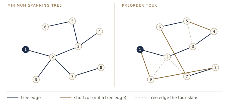
def mst_parents(D, root=0):
    """Prim's algorithm on the complete graph (array version).
    Returns the parent of each vertex in an MST rooted at root."""
    parent = {root: None}
    best = {v: (D[root][v], root) for v in range(len(D)) if v != root}
    while best:
        v = min(best, key=lambda u: best[u][0])
        parent[v] = best.pop(v)[1]
        for u in best:
            if D[v][u] < best[u][0]:
                best[u] = (D[v][u], v)
    return parent

def mst_tour(D):
    """2-approximate metric TSP tour: the preorder of an MST.
    Returns (tour, MST weight)."""
    parent = mst_parents(D)
    children = {v: [] for v in parent}
    for v, p in parent.items():
        if p is not None:
            children[p].append(v)
    tour, stack = [], [0]
    while stack:                           # iterative preorder traversal
        v = stack.pop()
        tour.append(v)
        stack.extend(reversed(children[v]))
    return tour, sum(D[v][p] for v, p in parent.items() if p is not None)

rng = random.Random(2026)
ratios = []
for _ in range(20):
    D = distance_matrix(random_points(9, rng))
    tour, mst = mst_tour(D)
    ours = tour_length(D, tour)
    opt, _, _ = tsp_branch_and_bound(D)
    assert sorted(tour) == list(range(9))
    assert mst <= opt <= ours <= 2 * mst + 1e-9
    ratios.append(ours / opt)
print(f"20 instances, n = 9: ratio worst {max(ratios):.3f}, "
      f"average {sum(ratios) / len(ratios):.3f}")
20 instances, n = 9: ratio worst 1.316, average 1.138
Again the typical ratio is far below the guarantee. Prim’s algorithm on the complete graph takes \(O(n^2)\) time and the traversal \(O(n)\), so the whole algorithm is \(O(n^2)\), linear in the size of the distance matrix. A cleverer algorithm by Christofides adds a minimum-weight perfect matching on the odd-degree vertices of the tree instead of doubling it, and guarantees a factor of 1.5.
General TSP cannot be approximated
Without the triangle inequality, shortcuts can be arbitrarily expensive, and the argument collapses. In fact, no argument can work. Recall the reduction from Rudrata cycle (a cycle through every vertex exactly once, also called a Hamiltonian cycle) to TSP in module 07. Given a graph \(G\) on \(n\) vertices and a number \(C > 0\), build the TSP instance \(I(G, C)\) on the same vertices with
\[d_{uv} = \begin{cases} 1 & \text{if } (u, v) \text{ is an edge of } G, \\ 1 + C & \text{otherwise.} \end{cases}\]If \(G\) has a Rudrata cycle, that cycle is a tour of length exactly \(n\), and no tour is shorter. If \(G\) has none, every tour uses at least one non-edge, so it costs at least \((n - 1) + (1 + C) = n + C\). There is nothing in between: the optimum is either \(n\) or at least \(n + C\). We can watch this gap on two six-vertex graphs: the triangular prism, which has a Rudrata cycle, and the complete bipartite graph \(K_{2,4}\), which has none (a cycle in a bipartite graph alternates sides, so it cannot pass through four vertices on one side using only two on the other).
def tsp_from_graph(G, C):
    """TSP instance I(G, C): distance 1 on edges of G, 1 + C elsewhere."""
    n = len(G)
    return [[0 if u == v else (1 if v in G[u] else 1 + C) for v in range(n)]
            for u in range(n)]

prism = {0: [1, 2, 3], 1: [0, 2, 4], 2: [0, 1, 5],     # two triangles, 0-1-2
         3: [0, 4, 5], 4: [1, 3, 5], 5: [2, 3, 4]}     # and 3-4-5, joined
k24 = {0: [2, 3, 4, 5], 1: [2, 3, 4, 5],
       2: [0, 1], 3: [0, 1], 4: [0, 1], 5: [0, 1]}
for name, G in [("prism", prism), ("K_2,4", k24)]:
    for C in [10, 1000]:
        opt, tour, _ = tsp_brute_force(tsp_from_graph(G, C))
        print(f"{name:6s} C = {C:5d}: optimal tour length {opt}")
prism  C =    10: optimal tour length 6
prism  C =  1000: optimal tour length 6
K_2,4  C =    10: optimal tour length 26
K_2,4  C =  1000: optimal tour length 2006
The prism’s optimum is 6 whatever \(C\) is. For \(K_{2,4}\) the optimum is \(6 + 2C\): a tour of \(K_{2,4}\)’s vertices needs at least two non-edges, so here the gap is even wider than the guaranteed \(C\). Making \(C\) large stretches the gap as far as we like, and that is what the proof below exploits.
Theorem. If P ≠ NP, then for no constant \(\alpha \ge 1\) is there a polynomial-time \(\alpha\)-approximation algorithm for the (general) TSP.
Proof. Suppose algorithm \(A\) were one. Given a graph \(G\) on \(n\) vertices, build \(I(G, C)\) with \(C = \alpha n\) and run \(A\) on it. If \(G\) has a Rudrata cycle, \(\mathrm{OPT} = n\) and \(A\) returns a tour of length at most \(\alpha n\). If not, every tour, including \(A\)’s, has length at least \(n + \alpha n > \alpha n\). So comparing \(A\)’s tour length with \(\alpha n\) decides whether \(G\) has a Rudrata cycle, in polynomial time. Rudrata cycle is NP-complete, so P = NP. \(\square\)
The same proof works when \(\alpha\) grows with \(n\), as long as \(\alpha n\) can be written down in polynomially many bits (for example \(\alpha = 2^n\)). The lesson is that the metric condition is not a technicality: it is exactly what separates a TSP that can be approximated from one that cannot.
Knapsack
We end the approximation algorithms with a maximization problem whose guarantee comes as close to exact as we like. Recall knapsack from module 06: there are \(n\) items with positive integer weights \(w_1, \dots, w_n\) and values \(v_1, \dots, v_n\), and we want the most valuable set of items with total weight at most \(W\). The dynamic program of module 06 runs in \(O(nW)\) time. That is not polynomial, because \(W\) is written with only \(\log W\) bits, so \(W\) can be exponential in the input size.
A second dynamic program indexes by value instead of weight. Let \(V = \sum_i v_i\), and for \(0 \le i \le n\) and \(0 \le s \le V\) let
\[A(i, s) = \text{the least total weight of a subset of items } 1, \dots, i \text{ with total value exactly } s\](or \(\infty\) if no subset has value \(s\)). Then \(A(0, 0) = 0\), \(A(0, s) = \infty\) for \(s > 0\), and item \(i\) is either left out or put in:
\[A(i, s) = \min\bigl(A(i-1, s),\; A(i-1, s - v_i) + w_i\bigr),\]where the second option is available only when \(s \ge v_i\). The answer is the largest \(s\) with \(A(n, s) \le W\), and the table has \((n + 1)(V + 1)\) entries, so the running time is \(O(nV)\). That is no better when the values are large. But values, unlike weights, can be rounded without making a solution infeasible.
def knapsack_by_weight(items, W):
    """Exact optimal value in O(nW) time (the DP of module 06)."""
    K = [0] * (W + 1)
    for w, v in items:
        for cap in range(W, w - 1, -1):   # downward: each item used once
            K[cap] = max(K[cap], K[cap - w] + v)
    return K[W]

def knapsack_by_value(items, W):
    """Exact 0/1 knapsack in O(nV) time, V = total value.
    Returns (indices of an optimal set of items, number of table entries)."""
    n, V = len(items), sum(v for _, v in items)
    A = [[math.inf] * (V + 1) for _ in range(n + 1)]
    A[0][0] = 0
    for i, (w, v) in enumerate(items, 1):
        for s in range(V + 1):
            A[i][s] = A[i - 1][s]
            if s >= v and A[i - 1][s - v] + w < A[i][s]:
                A[i][s] = A[i - 1][s - v] + w
    s = max(s for s in range(V + 1) if A[n][s] <= W)
    chosen = []
    for i in range(n, 0, -1):                # walk back through the table
        if A[i][s] != A[i - 1][s]:        # item i was needed to reach value s
            chosen.append(i - 1)
            s -= items[i - 1][1]
    return sorted(chosen), (n + 1) * (V + 1)
The approximation algorithm takes an accuracy parameter \(\epsilon > 0\) from the user:
- Discard every item with \(w_i > W\) (it can never be used).
- Let \(v_{\max}\) be the largest remaining value and \(\mu = \epsilon v_{\max} / n\).
- Replace each value by \(\hat v_i = \lfloor v_i / \mu \rfloor\).
- Solve the knapsack problem with the rounded values exactly, by the value-indexed dynamic program, and return that set of items.
In words: measure values in units of \(\mu\) and throw away the fractions. The weights are untouched, so the returned set is feasible.
Theorem. The algorithm runs in \(O(n^3/\epsilon)\) time and returns a set of items whose value is at least \((1 - \epsilon)\) times the optimum.
Proof. Running time. Each rounded value is at most \(v_{\max}/\mu = n/\epsilon\), so the rounded values sum to at most \(n^2/\epsilon\), and the dynamic program takes \(O(n \cdot n^2/\epsilon) = O(n^3/\epsilon)\) time.
Quality. Let \(S^*\) be an optimal set, of value \(K^*\), and let \(\hat S\) be the set we return, which is optimal for the rounded values. From the definition of the floor, \(v_i/\mu - 1 < \hat v_i \le v_i/\mu\). So
\[\sum_{i \in \hat S} v_i \;\ge\; \mu \sum_{i \in \hat S} \hat v_i \;\ge\; \mu \sum_{i \in S^*} \hat v_i \;\ge\; \mu \sum_{i \in S^*} \Bigl(\frac{v_i}{\mu} - 1\Bigr) \;\ge\; K^* - n\mu \;=\; K^* - \epsilon\, v_{\max}.\]The first step uses \(v_i \ge \mu \hat v_i\); the second, that \(\hat S\) is optimal for the rounded values and \(S^*\) is a feasible set; the third, the lower bound on \(\hat v_i\); the fourth, that \(S^*\) has at most \(n\) items. Finally, the single item of value \(v_{\max}\) fits in the knapsack on its own (we discarded the ones that do not), so \(K^* \ge v_{\max}\) and \(K^* - \epsilon v_{\max} \ge (1 - \epsilon) K^*\). \(\square\)
A family of algorithms that, for every \(\epsilon > 0\), comes within a factor \(1 - \epsilon\) of the optimum (or \(1 + \epsilon\), for minimization) in time polynomial in both \(n\) and \(1/\epsilon\) is called a fully polynomial-time approximation scheme (FPTAS). Knapsack has one. The price of more accuracy is only a proportional increase in running time: halving \(\epsilon\) doubles the size of the table.
To test it we need instances with large values (so that the exact \(O(nV)\) program is hopeless) but a small capacity (so that the \(O(nW)\) program can still supply the exact optimum for comparison).
def knapsack_fptas(items, W, eps):
    keep = [i for i, (w, v) in enumerate(items) if w <= W]
    n = len(keep)
    mu = eps * max(items[i][1] for i in keep) / n
    rounded = [(items[i][0], math.floor(items[i][1] / mu)) for i in keep]
    chosen, cells = knapsack_by_value(rounded, W)
    return [keep[j] for j in chosen], cells

rng = random.Random(9)
instances = []
for _ in range(50):
    items = [(rng.randint(1, 100), rng.randint(10**6, 10**8))
             for _ in range(20)]
    W = sum(w for w, _ in items) // 3
    instances.append((items, W, knapsack_by_weight(items, W)))

V = sum(v for _, v in instances[0][0])
print(f"exact value-indexed table for one instance: {21 * (V + 1):.1e} entries")
print("   eps   guarantee   worst ratio   not optimal   largest table")
for eps in [0.8, 0.5, 0.2, 0.1, 0.05]:
    worst, misses, biggest = 1.0, 0, 0
    for items, W, opt in instances:
        S, cells = knapsack_fptas(items, W, eps)
        assert sum(items[i][0] for i in S) <= W
        ratio = sum(items[i][1] for i in S) / opt
        worst, misses = min(worst, ratio), misses + (ratio < 1)
        biggest = max(biggest, cells)
    print(f"{eps:6.2f}   {1 - eps:9.2f}   {worst:11.4f}   {misses:8d}/50"
          f"   {biggest:13,d}")
exact value-indexed table for one instance: 2.0e+10 entries
   eps   guarantee   worst ratio   not optimal   largest table
  0.80        0.20        0.9947          6/50           6,636
  0.50        0.50        0.9972          4/50          10,689
  0.20        0.80        0.9985          3/50          27,027
  0.10        0.90        0.9997          1/50          54,201
  0.05        0.95        0.9997          1/50         108,633
On 50 random instances with 20 items each, every ratio is far above the guarantee \(1 - \epsilon\), and the table stays tiny next to the exact value-indexed table. The proof charges a rounding loss of up to \(\mu\) to each of up to \(n\) items and compares the total with \(v_{\max}\) alone. On typical instances the losses are smaller, and rounding rarely changes which set of items is best: even at \(\epsilon = 0.8\), 44 of the 50 answers are exactly optimal.
The approximability hierarchy
Put side by side, the examples fall into levels. Assuming P ≠ NP, NP-hard optimization problems range from those with no useful approximation to those that can be approximated as closely as we like:
| Level | What is possible in polynomial time | Examples |
|---|---|---|
| No constant ratio | no \(\alpha\)-approximation for any constant \(\alpha\) | general TSP |
| Logarithmic ratio | ratio about \(\log n\), and no constant ratio is known | set cover |
| Constant ratio | some constant \(\alpha > 1\), but not every \(\alpha\) close to 1 | vertex cover, \(k\)-cluster, metric TSP |
| Approximation scheme | ratio \(1 + \epsilon\) for every \(\epsilon > 0\) | knapsack (an FPTAS) |
For the constant-ratio problems the limits are real: for each of them there is a constant \(\alpha_0 > 1\) such that ratio \(\alpha_0\) is NP-hard to achieve, though the proofs are among the deepest results in complexity theory and well beyond this course.
Watch out. The whole hierarchy rests on the assumption P ≠ NP. If P = NP, every one of these problems can be solved exactly in polynomial time, and the levels collapse into one.
Two more lessons from the experiments. First, worst-case ratios are pessimistic: on random inputs, all our algorithms did much better than their guarantees. Second, an approximation algorithm is also a good starting point for the methods of the next section, which can take its answer and try to improve it.
Local search heuristics
The third strategy gives up on guarantees. Local search imitates a process of trial and error: start from some solution, make a small change, keep it if it helps, and repeat until no small change helps. For a minimization problem:
- Start from any solution \(s\).
- While some solution \(s'\) in the neighborhood of \(s\) has \(\mathrm{cost}(s') < \mathrm{cost}(s)\), replace \(s\) by \(s'\).
- Return \(s\).
The neighborhood — which solutions count as “a small change” from \(s\) — is not part of the problem; we impose it, and it is the central design decision. A solution with no better neighbor is a local optimum. The algorithm always stops at one (each step lowers the cost, and there are finitely many solutions), but a local optimum need not be a global one.
The traveling salesman problem, once more
For the TSP, a natural neighborhood is “tours that differ in few edges”. Two different tours cannot differ in exactly one edge: removing one edge from a tour leaves a path through all the cities, and the only way to close that path into a tour is to put the same edge back. So the smallest sensible change swaps two edges. The 2-change neighborhood of a tour consists of the tours obtained by deleting two of its edges and reconnecting the two resulting paths the other way.
Concretely, if the tour is \(t_0, t_1, \dots, t_{n-1}\) and we delete the edges \((t_i, t_{i+1})\) and \((t_j, t_{j+1})\) with \(i < j\), the only other way to reconnect is to add \((t_i, t_j)\) and \((t_{i+1}, t_{j+1})\), which amounts to reversing the segment \(t_{i+1}, \dots, t_j\). The change in length is
\[\Delta = d(t_i, t_j) + d(t_{i+1}, t_{j+1}) - d(t_i, t_{i+1}) - d(t_j, t_{j+1}),\]computed in constant time. There are \(n(n-3)/2\) pairs of non-adjacent edges, so a tour has \(O(n^2)\) neighbors. Local search with this neighborhood is known as 2-opt.
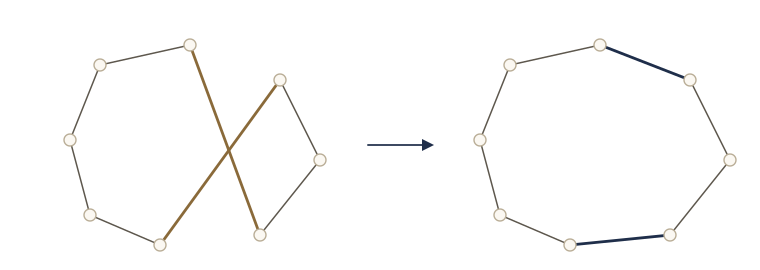
def two_opt(D, tour):
    """Local search with the 2-change neighborhood: apply improving
    2-changes (the first one found) until none is left.
    Returns (locally optimal tour, number of moves)."""
    tour, n, moves = tour[:], len(tour), 0
    improved = True
    while improved:
        improved = False
        for i in range(n - 1):
            # edges (t_i, t_i+1) and (t_j, t_j+1), which must not be adjacent
            for j in range(i + 2, n if i > 0 else n - 1):
                a, b, c, d = tour[i], tour[i + 1], tour[j], tour[(j + 1) % n]
                if D[a][c] + D[b][d] - D[a][b] - D[c][d] < -1e-12:
                    tour[i + 1:j + 1] = reversed(tour[i + 1:j + 1])
                    moves += 1
                    improved = True
    return tour, moves

def random_tour(n, rng):
    tour = list(range(n))
    rng.shuffle(tour)
    return tour

rng = random.Random(4)
runs = hits = 0
worst = 1.0
for _ in range(20):
    D = distance_matrix(random_points(9, rng))
    opt, _, _ = tsp_branch_and_bound(D)
    for _ in range(10):
        tour, _ = two_opt(D, random_tour(9, rng))
        ratio = tour_length(D, tour) / opt
        runs, hits = runs + 1, hits + (ratio < 1 + 1e-9)
        worst = max(worst, ratio)
print(f"n = 9: {hits} of {runs} runs end at an optimal tour; "
      f"worst ratio {worst:.3f}")
n = 9: 164 of 200 runs end at an optimal tour; worst ratio 1.072
How good is this procedure, by our two standard questions? Each iteration is fast: \(O(n^2)\) neighbors, each checked in \(O(1)\) time. But nothing in the algorithm bounds the number of iterations; there are instances on which 2-opt takes exponentially many improving moves. And all we know about the answer is that it is locally optimal. On the small instances above, most runs reach the true optimum and the others end close to it. On a larger instance, different random starts end at different local optima:
rng = random.Random(40)
D = distance_matrix(random_points(40, rng))
lengths, moves = [], []
for _ in range(20):
    tour, m = two_opt(D, random_tour(40, rng))
    lengths.append(tour_length(D, tour))
    moves.append(m)
approx, mst = mst_tour(D)
distinct = len(set(round(x, 6) for x in lengths))
print(f"20 runs of 2-opt, n = 40: {distinct} different local optima")
print(f"  lengths from {min(lengths):.1f} to {max(lengths):.1f}; "
      f"{min(moves)} to {max(moves)} moves per run")
print(f"  MST tour {tour_length(D, approx):.1f}; MST lower bound {mst:.1f}")
print("  best of first 1, 5, 20 runs: "
      + ", ".join(f"{min(lengths[:t]):.1f}" for t in [1, 5, 20]))
print(f"  best / MST lower bound = {min(lengths) / mst:.3f}")
20 runs of 2-opt, n = 40: 20 different local optima
  lengths from 558.4 to 647.6; 76 to 116 moves per run
  MST tour 724.0; MST lower bound 446.8
  best of first 1, 5, 20 runs: 634.5, 565.5, 558.4
  best / MST lower bound = 1.250
All twenty runs end at different tours, and every one of them is shorter than the tour from the 2-approximation. The best is about 1.25 times the MST lower bound, and therefore at most about 1.25 times the optimum (which we cannot compute here). Taking the best of several runs clearly helps.
A larger neighborhood can remove some poor local optima. The 3-change neighborhood deletes up to three edges and reconnects the pieces in any way; it can, for instance, move a single city from one place in the tour to another, which 2-change cannot always do in one step. But it has \(O(n^3)\) neighbors, so each iteration costs more, and it still has suboptimal local optima. This is the basic tradeoff of local search: small neighborhoods are fast to search but trap the search in more local optima; large ones trap it less but cost more per step. The right compromise is found by experiment.
Note. Local search is not guaranteed to do anything good, yet it is among the best-performing methods known for a wide range of optimization problems. The Lin–Kernighan heuristic for the TSP, a carefully engineered variable-depth version of \(k\)-change, is the core of many of the strongest practical TSP codes.
Graph partitioning
Graph partitioning asks to split a graph into two large pieces with few edges between them. The input is an undirected graph \(G = (V, E)\) with nonnegative edge weights and a number \(\alpha \in (0, 1/2]\). The output is a partition of \(V\) into two sets \(A\) and \(B\), each with at least \(\alpha \lvert V \rvert\) vertices, and the goal is to minimize the cut, the total weight of edges between \(A\) and \(B\). It arises in circuit layout (placing components so few wires cross between chips), in dividing work among processors, and in image segmentation. Without the size constraint this is the minimum cut problem, which is solvable in polynomial time with network flows (DPV chapter 7); with it the problem is NP-hard.
We focus on \(\alpha = 1/2\), bisection, where \(\lvert A \rvert = \lvert B \rvert\), and on unweighted edges. (The general problem reduces to this case, so nothing essential is lost.) A natural neighborhood: swap one vertex \(a \in A\) with one vertex \(b \in B\). There are \((n/2)^2\) such swaps. To evaluate one quickly, define the gain of a vertex \(x\) as the number of its neighbors on the other side minus the number on its own side: that is how much the cut would shrink if \(x\) alone switched sides. When \(a\) and \(b\) trade places, the cut shrinks by \(\mathrm{gain}(a) + \mathrm{gain}(b)\), except that an edge \((a, b)\) was counted as shrinking twice when in fact it stays cut; so the change in the cut is
\[\Delta = -\bigl(\mathrm{gain}(a) + \mathrm{gain}(b) - 2[(a, b) \in E]\bigr),\]where \([(a, b) \in E]\) is 1 if the edge exists and 0 otherwise.
def cut_size(G, A):
    return sum(1 for u in A for v in G[u] if v not in A)

def gain(G, A, x):
    """Decrease in the cut if x alone switched sides:
    neighbors on the other side minus neighbors on x's own side."""
    outside = sum(1 for y in G[x] if (y in A) != (x in A))
    return outside - (len(G[x]) - outside)

def swap_delta(G, A, a, b):
    """Change in the cut if a (in A) and b (not in A) trade sides."""
    return -(gain(G, A, a) + gain(G, A, b) - 2 * (b in G[a]))

def random_bisection(G, rng):
    V = list(G)
    rng.shuffle(V)
    return set(V[:len(V) // 2])

def swap_local_search(G, A):
    """Make improving swaps (the first found) until none is left.
    Returns (A, cut, number of swaps evaluated)."""
    A, cut, evaluated = set(A), cut_size(G, A), 0
    while True:
        B = [v for v in G if v not in A]
        move = None
        for a in sorted(A):
            for b in B:
                evaluated += 1
                if swap_delta(G, A, a, b) < 0:
                    move = (a, b)
                    break
            if move:
                break
        if move is None:
            return A, cut, evaluated
        a, b = move
        cut += swap_delta(G, A, a, b)
        A.remove(a)
        A.add(b)

def bisection_brute_force(G):
    """Smallest cut over all bisections (0 stays in A: no mirror images)."""
    n = len(G)
    return min(cut_size(G, {0, *rest})
               for rest in itertools.combinations(range(1, n), n // 2 - 1))

rng = random.Random(1)
G = random_graph(16, 0.3, rng)
opt = bisection_brute_force(G)
results = [swap_local_search(G, random_bisection(G, rng)) for _ in range(200)]
cuts = [cut for _, cut, _ in results]
print(f"{len(edges(G))} edges; optimal bisection cut = {opt}")
print(f"200 runs of swap local search: local optima with cuts "
      f"{sorted(set(cuts))}")
print(f"optimal in {sum(c == opt for c in cuts)} of 200 runs; "
      f"about {sum(e for *_, e in results) / 200:.0f} swaps evaluated per run")
32 edges; optimal bisection cut = 8
200 runs of swap local search: local optima with cuts [8, 9, 10, 11, 12]
optimal in 65 of 200 runs; about 146 swaps evaluated per run
This graph has \(\binom{16}{8}/2 = 6435\) bisections, few enough to check them all. Swap local search is fast, but it often stops at a local optimum that is not the global one.
Dealing with local optima
Randomization and restarts
Randomness enters local search in two places: in the starting solution, and in the choice among several improving moves. Its main benefit is that it lets us restart: run the search many times from independent random starts and keep the best result. If a single run reaches a good solution with probability \(p\), then \(t\) independent runs all miss it with probability
\[(1 - p)^t \le e^{-pt},\]so about \((1/p)\ln(1/\delta)\) runs suffice to succeed with probability at least \(1 - \delta\). For the graph above we can measure \(p\) from the 200 runs and check the formula by grouping the runs into batches of ten:
p = sum(c == opt for c in cuts) / len(cuts)
batches = [cuts[i:i + 10] for i in range(0, 200, 10)]
misses = sum(min(b) > opt for b in batches)
print(f"p = {p:.3f}; chance 10 runs all miss: (1 - p)^10 = {(1 - p)**10:.3f}")
print(f"batches of 10 runs that never found the optimum: {misses} of 20")
p = 0.325; chance 10 runs all miss: (1 - p)^10 = 0.020
batches of 10 runs that never found the optimum: 1 of 20
One batch in twenty is a 5 percent rate, against a prediction of 2 percent; with only twenty batches, that difference is well within chance.
Restarts are cheap and effective when \(p\) is not too small. The trouble is that on larger instances bad local optima tend to vastly outnumber good ones, and \(p\) can shrink exponentially with the size of the input. Then restarting is hopeless and something else is needed.
Simulated annealing
The other remedy is to let the search go uphill now and then, so that it can climb out of a poor local optimum. Simulated annealing does this in a controlled way, using a parameter \(T > 0\) called the temperature:
- Start from any solution \(s\).
- Repeat: pick a random neighbor \(s'\) of \(s\) and let \(\Delta = \mathrm{cost}(s') - \mathrm{cost}(s)\). If \(\Delta < 0\), move to \(s'\). Otherwise move to \(s'\) with probability \(e^{-\Delta/T}\).
At \(T = 0\) uphill moves are never accepted, and this is ordinary local search with random moves. At high temperature, uphill moves are accepted often: a move that costs 2 is taken with probability \(e^{-1} \approx 0.37\) when \(T = 2\), but with probability \(e^{-4} \approx 0.02\) when \(T = 0.5\). The idea is to start hot, so the search wanders widely with only a mild preference for low cost, and to cool slowly, so it settles into ever lower regions and finally freezes into a local optimum that is, with luck, a very good one. The name comes from metallurgy: a metal cooled slowly (annealed) has time for its atoms to settle into a low-energy, well-ordered arrangement, while a metal cooled quickly freezes into a disordered one.
The rule for lowering the temperature is the annealing schedule. A common choice, used below, is geometric cooling: multiply \(T\) by a constant slightly below 1 after every step.
def anneal_bisection(G, A, rng, T=2.0, cooling=0.995, steps=3000):
    """Simulated annealing over bisections: random swaps, geometric cooling."""
    A = set(A)
    cut = cut_size(G, A)
    for _ in range(steps):
        a = rng.choice(sorted(A))
        b = rng.choice([v for v in G if v not in A])
        delta = swap_delta(G, A, a, b)
        if delta < 0 or rng.random() < math.exp(-delta / T):
            A.remove(a)
            A.add(b)
            cut += delta
        T *= cooling
    return A, cut

rng = random.Random(2)
sa_cuts = [anneal_bisection(G, random_bisection(G, rng), rng)[1]
           for _ in range(20)]
print(f"20 annealing runs (3000 swaps evaluated each): "
      f"final cuts {sorted(set(sa_cuts))}")
print(f"optimal in {sum(c == opt for c in sa_cuts)} of 20")
20 annealing runs (3000 swaps evaluated each): final cuts [8]
optimal in 20 of 20
All 20 annealing runs finish at the optimum, while a single run of plain local search gets there only about a third of the time. The price is time: an annealing run evaluates 3000 swaps, about twenty times as many as one run of plain local search, so the fair comparison is with a batch of about twenty restarts — and by the formula above, twenty restarts would also almost surely find the optimum of this small graph. The case for annealing is on large instances, where \(p\) is tiny and restarts stop working.
Watch out. Simulated annealing has no general guarantee, and its schedule is a matter of tuning: cool too fast and it behaves like plain local search, cool too slowly and it wastes time wandering. The starting temperature, the cooling factor, and the number of steps all have to be chosen by experiment for each kind of instance (exercise 11).
Summary
| Problem | Method | Guarantee | Running time |
|---|---|---|---|
| SAT | backtracking, branching on a shortest clause | exact | exponential in the worst case |
| TSP | branch and bound with the MST lower bound | exact | exponential in the worst case |
| Vertex cover | endpoints of a maximal matching | at most \(2 \cdot \mathrm{OPT}\) | \(O(n + m)\) |
| \(k\)-cluster (metric) | farthest-first traversal | at most \(2 \cdot \mathrm{OPT}\) | \(O(nk)\) distance evaluations |
| Metric TSP | preorder of a minimum spanning tree | at most \(2 \cdot \mathrm{OPT}\) | \(O(n^2)\) |
| General TSP | none possible | no constant ratio unless P = NP | — |
| Knapsack | round the values, dynamic program by value | at least \((1 - \epsilon) \cdot \mathrm{OPT}\) | \(O(n^3/\epsilon)\) |
| TSP, bisection | local search (2-change, swaps), restarts, simulated annealing | none | polynomial per step; number of steps unbounded |
Ideas to carry forward:
- An NP-completeness proof is the start of the design process, not the end. Check first for a special case that is easy.
- Exhaustive search can be made intelligent by pruning, and the pruning is only as good as the test or the lower bound behind it.
- To prove an approximation ratio without knowing the optimum, find a structure that is both cheap to compute and a lower bound on the optimum (a matching, \(k + 1\) well-separated points, a spanning tree), and build the solution from it.
- Local search needs a well-chosen neighborhood and a way out of poor local optima; its value is established by experiment, not proof.
Looking back over the course
We started in module 00 with three questions — is it correct, how long does it take, can we do better — and a Fibonacci algorithm that was exponentially slower than it needed to be. Module 01 counted bit operations in arithmetic and built RSA and primality testing from them. Module 02 split problems in half and solved recurrences with the master theorem. Modules 03 and 04 explored graphs with depth-first and breadth-first search and found shortest paths. Module 05 showed when a sequence of locally best choices is globally optimal, and module 06 solved each subproblem once and stored the answer. Module 07 turned the question around and gave strong evidence that for many natural problems no such technique will ever give a fast exact algorithm. This module showed that the design techniques do not stop there: the MST from module 05 became a lower bound and a tour, depth-first search became backtracking, and the knapsack dynamic program became an approximation scheme. The three questions still apply; only the answers have become more nuanced — “correct” may mean “within a factor of 2”, and “fast” may mean “fast on the inputs we actually see”.
Exercises
- Suppose every clause of a formula has at most two literals (2SAT). Show that when
backtrack_satsets a variable on such a formula, the forced settings that follow (one-literal clauses) either produce an empty clause within \(n\) further steps or leave a formula that is a subset of the original clauses. Use this to show that the search tests only polynomially many subproblems. - Replace the MST lower bound in
tsp_branch_and_boundby the cost of the path so far, and by the path cost plus the two lightest edges alone (no MST). Compare the number of partial tours generated on the instances of the code above. Then add a second check that discards a partial tour when it is popped if its bound is no longer belowbest_so_far. Does it help? - Explain why choosing the deepest active partial tour first (a stack) is a good choice for branch and bound, while choosing the shallowest (a queue) is a bad one. What is the argument for choosing the partial tour with the smallest lower bound instead?
- For every \(k \ge 1\), give a graph on which every maximal matching produces a vertex cover exactly twice the optimum. Then give a graph on which greedy vertex cover (take a vertex of highest degree, delete it with its edges, repeat) returns more than twice the optimum.
- The complement \(V - S\) of a vertex cover \(S\) is an independent set. Show that the vertex cover algorithm does not give an approximation algorithm with any constant ratio for maximum independent set, by finding graphs where the complement of its cover is tiny while the largest independent set is large.
- Place four points on a line so that farthest-first traversal with \(k = 2\), started from a badly chosen point, returns a clustering whose diameter is nearly twice the optimum. Does the result depend on the starting point?
- In the metric TSP algorithm, prove that the preorder tour is exactly what shortcutting the doubled depth-first walk produces. Then search randomly, with the code of this module, for small instances in the plane on which
mst_tourdoes as badly as you can make it. How close to 2 can you get, and what do the bad instances look like? - In the knapsack approximation scheme, where exactly does the proof use the fact that items heavier than \(W\) were discarded? Give an instance showing that without this step the algorithm can return a solution worth much less than \((1 - \epsilon)\mathrm{OPT}\).
- Prove that for cities in the plane with Euclidean distances, a tour that 2-opt cannot improve has no two crossing edges. Is the converse true: is every tour without crossings 2-opt-optimal?
- Max cut asks for a partition of the vertices into two sets (of any sizes) that maximizes the number of edges between them. Consider local search that moves one vertex to the other side whenever that increases the cut. Show that at a local optimum each vertex has at least half of its edges crossing the cut, and conclude that this is a 2-approximation. How many moves can it make at most?
- Run
anneal_bisectionon the graph of this module with cooling factors 0.9, 0.99, 0.995, and 0.999 (adjust the number of steps so that the final temperature is about the same). How does the fraction of runs that reach the optimum change? Compare with plain local search given the same total number of swap evaluations. - In your own words: a colleague has shown that the scheduling problem at their company is NP-complete and concludes that the software should just use a simple rule of thumb. Describe the three strategies of this module and what each would offer them, and what questions about their instances would help decide among them.
Going further
- Dasgupta, Papadimitriou, and Vazirani, Algorithms, chapter 9 and its exercises 9.1–9.10 — the source for this module. Exercise 9.1 is the 2SAT claim of exercise 1 above, 9.5 studies local search for spanning trees, and 9.8 approximates MAX SAT by flipping coins.
- David P. Williamson and David B. Shmoys, The Design of Approximation Algorithms (Cambridge University Press, 2011) — a full textbook on approximation algorithms, including Christofides’ algorithm and approximation schemes; the authors provide an electronic version on the book’s site.
- T. F. Gonzalez, “Clustering to minimize the maximum intercluster distance”, Theoretical Computer Science 38 (1985) — the farthest-first traversal and the matching hardness result for \(k\)-cluster.
- B. W. Kernighan and S. Lin, “An efficient heuristic procedure for partitioning graphs”, Bell System Technical Journal, 1970 — the classic local search for graph partitioning, with a neighborhood built from sequences of swaps.
- S. Kirkpatrick, C. D. Gelatt, and M. P. Vecchi, “Optimization by simulated annealing”, Science, 1983 — the paper that introduced simulated annealing for combinatorial optimization.
These notes follow the chapters of S. Dasgupta, C. H. Papadimitriou, and U. V. Vazirani, Algorithms (McGraw-Hill, 2008), the course text. The explanations, code, figures, and exercises here are written for this course; the book remains the reference, with many more exercises.