CSE 431/531 · Module 03 · Week 3
Decompositions of Graphs
Representing graphs, depth-first search, pre/post numbers, DAGs and topological order, strongly connected components.
Companion reading: Dasgupta, Papadimitriou & Vazirani, Algorithms, chapter 3, “Decompositions of graphs”
By the end of this module you can
- Model a problem as a graph, and choose between an adjacency matrix and adjacency lists by comparing their space and time costs for sparse and dense graphs.
- Run depth-first search by hand and in code, recording pre and post numbers, and prove that it finds exactly the vertices reachable from its start in \(O(n + m)\) time.
- Use depth-first search to find the connected components of an undirected graph.
- Classify the edges of a directed graph as tree, forward, back, or cross edges from their pre and post numbers alone.
- Prove that a directed graph has a cycle if and only if depth-first search finds a back edge, and topologically sort a DAG by decreasing post number.
- Explain why every directed graph is a DAG of its strongly connected components, and find those components in linear time with two depth-first searches.
- Recognize when recursion depth becomes a problem in Python and replace recursive search with an explicit stack.
Contents
- Why graphs
- Depth-first search in undirected graphs
- Depth-first search in directed graphs
- Strongly connected components
- Depth-first search without recursion
- Summary
- Exercises
- Going further
In module 02 the input was a list or a number, and the art was in splitting it into smaller pieces of the same kind. From here to module 06 the input is usually a graph: a set of objects and the pairwise connections between them. Graphs describe road networks, links between web pages, prerequisites between courses, conflicts between exams, and a great many problems that do not look like graph problems at first.
This module is about the most basic question you can ask of a graph: how is it connected? What can be reached from where, which parts hang together, and in what order can the parts be visited? One procedure answers all of these, depth-first search, and it does so in time proportional to the size of the graph. We develop it for undirected graphs first, then for directed graphs, where it detects cycles, orders tasks that depend on one another, and splits any directed graph into its strongly connected components. Modules 04–06 build on the representation and the code written here.
Why graphs
Problems that are graphs in disguise
Suppose a department has to schedule final exams and wants as few time slots as possible. The only rule is that two exams cannot share a slot if some student takes both. Draw one point per exam and join two points by a line whenever the exams share a student. Now forget the students: all the scheduling problem needs is this picture. A schedule is a way of labeling the points with slot numbers so that no line joins two points with the same label.
The same picture describes coloring a map (one point per country, a line between countries that share a border, colors instead of slots), assigning radio frequencies to transmitters that would interfere, and assigning registers to program variables that are alive at the same time. Stripping a problem down to its points and lines removes everything that does not matter and makes the common structure visible. That is the reason graphs are everywhere in algorithms.
Here is the exam problem in code. Each student lists their exams; two exams conflict if they appear on the same list.
from itertools import combinations, product

# Which exams each student is taking (a small made-up term).
enrolled = {
    "ana":  ["algo", "stats", "ml"],
    "ben":  ["algo", "db"],
    "chen": ["stats", "db"],
    "dara": ["ml", "os"],
    "eli":  ["db", "nets", "os"],
    "femi": ["nets", "algo"],
}

def conflict_graph(enrolled):
    """One vertex per exam; an edge between two exams that share a student."""
    G = {}
    for exams in enrolled.values():
        for e in exams:
            G.setdefault(e, [])
        for a, b in combinations(exams, 2):
            if b not in G[a]:
                G[a].append(b)
                G[b].append(a)
    return G

exams = conflict_graph(enrolled)
for e in sorted(exams):
    print(f"{e:>5}: {sorted(exams[e])}")
 algo: ['db', 'ml', 'nets', 'stats']
   db: ['algo', 'nets', 'os', 'stats']
   ml: ['algo', 'os', 'stats']
 nets: ['algo', 'db', 'os']
   os: ['db', 'ml', 'nets']
stats: ['algo', 'db', 'ml']
A coloring with \(k\) colors gives every vertex one of \(k\) labels so that the two ends of each edge get different labels. The smallest number of slots is the smallest \(k\) for which a coloring exists. For six exams we can afford to try every labeling:
def fewest_colors(G):
    """Smallest k with a proper k-coloring, by trying all k^n labelings."""
    V = list(G)
    for k in range(1, len(V) + 1):
        for labels in product(range(k), repeat=len(V)):
            color = dict(zip(V, labels))
            if all(color[u] != color[v] for u in G for v in G[u]):
                return k, color

k, slot = fewest_colors(exams)
print(k, "slots:", {s: sorted(e for e in slot if slot[e] == s) for s in range(k)})
3 slots: {0: ['algo', 'os'], 1: ['nets', 'stats'], 2: ['db', 'ml']}
Three slots suffice, and no schedule can do with two: algo, db, and stats conflict pairwise (through ana, ben, and chen), so they need three different slots.
Note. Trying all \(k^n\) labelings is exponential, and for coloring nobody knows how to do fundamentally better: deciding whether a graph can be colored with 3 colors is NP-complete, as we will see in module 07. This module is about the opposite kind of problem, questions about connectivity that can be answered in linear time.
Vocabulary
A graph \(G = (V, E)\) is a set \(V\) of vertices (also called nodes) and a set \(E\) of edges between pairs of vertices. Throughout the course, \(n = \lvert V \rvert\) and \(m = \lvert E \rvert\).
- In an undirected graph an edge \(\{u, v\}\) is a symmetric connection: “exam \(u\) conflicts with exam \(v\)” means the same as the reverse. The neighbors of \(u\) are the vertices joined to it, and the degree of \(u\) is the number of its neighbors.
- In a directed graph an edge \((u, v)\) goes from \(u\) to \(v\): “page \(u\) links to page \(v\)”, “course \(u\) is a prerequisite of course \(v\)”. The two directions are different edges, and a graph may have one, the other, or both.
- A path from \(u\) to \(v\) is a sequence of vertices \(u = v_0, v_1, \dots, v_k = v\) with an edge from each \(v_{i-1}\) to \(v_i\); its length is \(k\), the number of edges. If such a path exists, \(v\) is reachable from \(u\). A cycle is a path of length at least 1 that ends where it started (in an undirected graph we also require at least three distinct vertices, so that going along one edge and straight back does not count).
We assume graphs have no repeated edges. Many algorithms in this module work unchanged for both kinds of graph; when that is the case we write edges as \((u, v)\) and think of an undirected edge as a pair of directed edges, one each way.
Representing a graph
There are two standard ways to store a graph. Number the vertices \(v_1, \dots, v_n\).
The adjacency matrix is an \(n \times n\) array \(A\) with \(a_{ij} = 1\) if there is an edge from \(v_i\) to \(v_j\) and \(a_{ij} = 0\) otherwise. For an undirected graph the matrix is symmetric.
The adjacency list representation stores, for each vertex \(u\), a list of the vertices \(v\) with an edge \((u, v)\). A directed edge appears in one list; an undirected edge \(\{u, v\}\) appears in two, \(v\) in the list of \(u\) and \(u\) in the list of \(v\). In Python a dictionary of lists is the natural form, and it is the form we use for the rest of the course: G[u] is the list of u’s neighbors, and every vertex is a key, even one with no edges.
def graph(edges, vertices=(), directed=False):
    """Adjacency lists {u: [v, ...]} built from a list of edges (u, v).
    Every vertex is a key, isolated ones included. Vertices and neighbor lists are
    sorted, so that every search below breaks ties in alphabetical order."""
    G = {v: [] for v in vertices}
    for u, v in edges:
        G.setdefault(u, [])
        G.setdefault(v, [])
        G[u].append(v)
        if not directed:
            G[v].append(u)
    return {u: sorted(G[u]) for u in sorted(G)}

def adjacency_matrix(G):
    """The same graph as a 0/1 matrix, with the vertices in the order of G's keys."""
    index = {v: i for i, v in enumerate(G)}
    A = [[0] * len(G) for _ in G]
    for u in G:
        for v in G[u]:
            A[index[u]][index[v]] = 1
    return A

small = graph([("a", "b"), ("a", "c"), ("b", "c"), ("c", "d")], vertices=["e"])
print(small)
for row in adjacency_matrix(small):
    print(row)
{'a': ['b', 'c'], 'b': ['a', 'c'], 'c': ['a', 'b', 'd'], 'd': ['c'], 'e': []}
[0, 1, 1, 0, 0]
[1, 0, 1, 0, 0]
[1, 1, 0, 1, 0]
[0, 0, 1, 0, 0]
[0, 0, 0, 0, 0]
Vertex e has no edges: it is a key with an empty list, and its row and column of the matrix are all zeros. The two representations have different strengths:
| Operation | Adjacency matrix | Adjacency lists |
|---|---|---|
| space | \(\Theta(n^2)\) | \(\Theta(n + m)\) |
| is \((u, v)\) an edge? | \(O(1)\), one array lookup | \(O(\deg u)\), scan \(u\)’s list |
| list the neighbors of \(u\) | \(\Theta(n)\), scan a whole row | \(O(\deg u)\) |
| visit every edge once | \(\Theta(n^2)\) | \(\Theta(n + m)\) |
The algorithms in this module never ask “is \((u, v)\) an edge?”; they ask “what are the neighbors of \(u\)?”, over and over. That makes adjacency lists the right choice, and it is why their running times come out as \(O(n + m)\).
Note. In the dictionary form,
v in G[u]scans a list and costs \(O(\deg u)\). If an algorithm needs fast edge queries as well, store each vertex’s neighbors in a Pythonsetinstead of a list: a set lookup takes constant expected time, by the hashing of module 01. The price is that sets have no fixed order, which makes searches harder to follow by hand.
How big is your graph?
An undirected graph on \(n\) vertices has at most \(\binom{n}{2} = n(n-1)/2\) edges, and a directed one at most \(n(n-1)\); either way \(m = O(n^2)\). At the other end, a connected graph needs at least \(n - 1\) edges. A graph is called dense when \(m\) is close to the upper end, a constant fraction of \(n^2\), and sparse when \(m\) is close to \(n\), say \(O(n)\) or \(O(n \log n)\).
Most large graphs met in practice are sparse: a road network has a handful of roads at each intersection, and a web page links to a few dozen pages out of billions. For a sparse graph the gap between \(n^2\) and \(n + m\) is enormous. Take a directed graph with a billion vertices and ten edges per vertex:
n, per_vertex = 10**9, 10
matrix_bytes = n * n / 8               # one bit per matrix entry
list_bytes = n * per_vertex * 8        # one 8-byte vertex id per list entry
print(f"adjacency matrix: {matrix_bytes / 1e15:,.0f} petabytes")
print(f"adjacency lists:  {list_bytes / 1e9:,.0f} gigabytes")
adjacency matrix: 125 petabytes
adjacency lists:  80 gigabytes
The matrix does not fit in any single computer’s memory; the lists fit on a laptop’s disk. The same gap shows up in running time: an algorithm that looks at every matrix entry does \(10^{18}\) steps before it has done anything useful. Whether a graph is sparse or dense will keep influencing our choices, here and in the next three modules.
Depth-first search in undirected graphs
Exploring from one vertex
The most basic connectivity question is:
Given a graph \(G\) and a vertex \(s\), which vertices are reachable from \(s\)?
Imagine that you are the algorithm and all you can do is stand at a vertex and look at its list of neighbors. The situation is like walking through a cave system with many junctions. Two things keep you from getting lost. First, you mark each junction when you reach it, so that you never explore it twice and never walk in circles. Second, you remember the way you came in, so that when every passage from the current junction leads somewhere already marked, you can back up to the previous junction and try its remaining passages.
On a computer the marks are a set of visited vertices, and “the way back” is a stack of the junctions we are in the middle of exploring. Recursion keeps that stack for us: each call is a junction, and returning from the call is backing up.
def explore(G, v, visited=None):
    """Visit every vertex reachable from v; return the set of visited vertices."""
    if visited is None:
        visited = set()
    visited.add(v)
    for u in G[v]:
        if u not in visited:
            explore(G, u, visited)
    return visited
Here is the undirected graph we will use for the rest of this section. It has ten vertices and three pieces.
U = graph([("A", "B"), ("A", "D"), ("B", "C"), ("B", "D"), ("B", "E"), ("C", "E"),
           ("F", "G"), ("F", "H"), ("G", "H"), ("H", "I")], vertices=["J"])
for s in ["A", "H", "J"]:
    print(s, "reaches", sorted(explore(U, s)))
A reaches ['A', 'B', 'C', 'D', 'E']
H reaches ['F', 'G', 'H', 'I']
J reaches ['J']
Why explore is correct
Two things must be shown: explore visits nothing it should not, and it misses nothing it should visit.
Lemma.
explore(G, s)visits exactly the vertices reachable from \(s\).
The first half is immediate: explore only ever moves from a vertex to one of its neighbors, so every vertex it visits is at the end of a path from \(s\).
For the second half, the idea is that the first missed vertex on a path would have to be the neighbor of a visited vertex, and explore checks every neighbor of every vertex it visits. In detail: suppose \(u\) is reachable from \(s\) but not visited. Fix a path \(s = v_0, v_1, \dots, v_k = u\). Its first vertex is visited and its last is not, so there is a first index \(i\) with \(v_i\) visited and \(v_{i+1}\) not visited. But the call explore(G, v_i) ran the loop over all neighbors of \(v_i\), including \(v_{i+1}\); at that moment \(v_{i+1}\) was either already visited or got visited by the recursive call. Either way it is visited, a contradiction.
This “look at the first place where the claim fails” argument is induction in disguise: it is the same as proving, for \(k = 0, 1, 2, \dots\), that every vertex at distance \(k\) from \(s\) is visited. We will use it often.
Depth-first search of the whole graph
explore only sees the part of the graph reachable from its start. To visit everything, restart it from any vertex not yet visited, until none is left. That is depth-first search (DFS). While we are at it, we record two moments in the life of each vertex, using a counter clock that ticks once per event:
pre[v], the timevis first reached (the previsit), andpost[v], the timeexplorefinally leavesv(the postvisit).
We also record parent[v], the vertex from which v was discovered, and ccnum[v], the number of the restart that reached v. The function below is the workhorse of the module; later sections only add to what it returns.
from collections import namedtuple

Search = namedtuple("Search", "pre post parent ccnum finish")

def dfs(G, order=None):
    """Depth-first search of all of G, restarting in the given vertex order
    (default: the order of G's keys). Returns a Search with
      pre[v], post[v]  clock times when v is first reached and finally left,
      parent[v]        the vertex that discovered v (None if v started a new tree),
      ccnum[v]         the number of the restart (1, 2, ...) that reached v,
      finish           all vertices in the order they were postvisited."""
    pre, post, parent, ccnum, finish = {}, {}, {}, {}, []
    clock = 1
    cc = 0

    def explore(v):
        nonlocal clock
        pre[v] = clock; clock += 1           # previsit
        ccnum[v] = cc
        for u in G[v]:
            if u not in pre:                 # "visited" means "has a pre number"
                parent[u] = v
                explore(u)
        post[v] = clock; clock += 1          # postvisit
        finish.append(v)

    for v in (G if order is None else order):
        if v not in pre:
            cc += 1
            parent[v] = None
            explore(v)
    return Search(pre, post, parent, ccnum, finish)

S = dfs(U)
for v in U:
    print(f"{v}: pre {S.pre[v]:2d}  post {S.post[v]:2d}",
          f" parent {S.parent[v]}  ccnum {S.ccnum[v]}")
A: pre  1  post 10  parent None  ccnum 1
B: pre  2  post  9  parent A  ccnum 1
C: pre  3  post  6  parent B  ccnum 1
D: pre  7  post  8  parent B  ccnum 1
E: pre  4  post  5  parent C  ccnum 1
F: pre 11  post 18  parent None  ccnum 2
G: pre 12  post 17  parent F  ccnum 2
H: pre 13  post 16  parent G  ccnum 2
I: pre 14  post 15  parent H  ccnum 2
J: pre 19  post 20  parent None  ccnum 3
Follow the run in the figure below. The search starts at A, goes to B (the first neighbor of A), then to C, then to E. Every neighbor of E is already visited, so E is finished at time 5 and the search backs up to C, which is also finished, then to B, which still has an unvisited neighbor D. After D, B and then A are finished at time 10. The first restart has found everything reachable from A. The next restart is at F, and the last at the isolated vertex J.
Each call explore(u) made from inside explore(v) uses the edge \(\{v, u\}\) to reach a new vertex. These edges are the tree edges: every vertex except a restart point has exactly one, the edge to its parent, so they form a tree (a connected graph with no cycles) for each restart. The trees together form the DFS forest. The other edges, which led to vertices already visited, are back edges; A–D, B–E, and F–H are the back edges here.
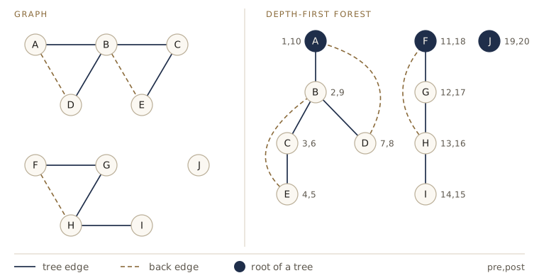
U, breaking ties alphabetically. Each tree edge led to a new vertex; each dashed back edge led to a vertex already on the current path. The numbers are pre and post times.Note. In an undirected graph every non-tree edge joins a vertex to one of its ancestors in the forest; there are no edges between different branches. (If
uwas discovered first and{u, v}is an edge, thenvmust be reached beforeexplore(u)finishes, sovlands belowu.) This is exercise 2, and it is the property that makes undirected graphs simpler than directed ones.
Running time
Each vertex is explored exactly once: explore(v) is called only when v has no pre number, and it gives v one immediately. The work in one call is a constant amount (the pre and post bookkeeping) plus one pass over G[v]. Summed over all vertices, the constant parts give \(O(n)\), and the passes over the lists touch each list entry once, \(\sum_v \deg v = 2m\) entries for an undirected graph and \(m\) for a directed one. So
linear time: proportional to the size of the adjacency lists, which is also the time it takes merely to read the input. We cannot hope to do better. The count is easy to confirm on a random graph:
import random

def random_graph(n, m, directed=False, rng=random):
    """A random graph on vertices 0..n-1 with m distinct edges and no self-loops
    (m is capped at the largest possible number of edges)."""
    m = min(m, n * (n - 1) if directed else n * (n - 1) // 2)
    edges = set()
    while len(edges) < m:
        u, v = rng.randrange(n), rng.randrange(n)
        if u != v and (directed or (v, u) not in edges):
            edges.add((u, v))
    return graph(sorted(edges), range(n), directed)

def dfs_counts(G):
    """Number of explore calls and of adjacency-list entries scanned by DFS."""
    calls = scans = 0
    visited = set()
    def explore(v):
        nonlocal calls, scans
        calls += 1
        visited.add(v)
        for u in G[v]:
            scans += 1
            if u not in visited:
                explore(u)
    for v in G:
        if v not in visited:
            explore(v)
    return calls, scans

random.seed(3)
R = random_graph(400, 1500)
calls, scans = dfs_counts(R)
print(f"n = 400, m = 1500:  explore calls = {calls}, list entries scanned = {scans}")
n = 400, m = 1500: explore calls = 400, list entries scanned = 3000
Exactly \(n\) calls and \(2m\) scans, as the argument says.
Watch out. Python limits recursion depth, by default to 1000 nested calls.
dfsnests one call per vertex on the current path, so on a graph with a long path (a chain of 5000 vertices, or a big random graph) it stops with aRecursionErrorrather than returning an answer. The notes keep the examples small; the section Depth-first search without recursion at the end shows the fix.
Connected components
An undirected graph is connected if every vertex is reachable from every other. U is not: nothing connects A to F. It splits into connected components, maximal sets of vertices that are reachable from one another: here \(\{A, B, C, D, E\}\), \(\{F, G, H, I\}\), and \(\{J\}\). Each edge lies inside one component, and no edge joins two components.
By the lemma, one call of explore visits exactly the component of its starting vertex. So each restart in dfs finds one new component, and ccnum[v] already names the component of v. Grouping by it gives the components in linear time:
def components(G):
    """Connected components of an undirected graph, as a list of vertex lists."""
    S = dfs(G)
    groups = {}
    for v in G:
        groups.setdefault(S.ccnum[v], []).append(v)
    return list(groups.values())

print(components(U))
[['A', 'B', 'C', 'D', 'E'], ['F', 'G', 'H', 'I'], ['J']]
The claim deserves a test against a slower method we trust more: u and v are in the same component exactly when v is in explore(G, u).
def same_component_brute(G):
    """For every pair, whether one reaches the other, by one explore per vertex."""
    reach = {u: explore(G, u) for u in G}
    return {(u, v): v in reach[u] for u in G for v in G}

random.seed(11)
agree = 0
for trial in range(200):
    n = random.randint(1, 30)
    R = random_graph(n, random.randint(0, n + 5))
    cc = dfs(R).ccnum
    brute = same_component_brute(R)
    agree += all((cc[u] == cc[v]) == same for (u, v), same in brute.items())
print(agree, "of 200 random graphs agree")
200 of 200 random graphs agree
Pre and post numbers: the parenthesis property
Write the life of each vertex as an interval \([\text{pre}(v), \text{post}(v)]\) on the clock. In the run above, \(A\) lives during \([1, 10]\), \(B\) during \([2, 9]\), \(D\) during \([7, 8]\), and \(F\) during \([11, 18]\). The intervals of \(B\) and \(D\) sit inside the interval of \(A\), and the interval of \(F\) is disjoint from all three. That is no accident.
Lemma (parenthesis property). For any two vertices \(u\) and \(v\), the intervals \([\text{pre}(u), \text{post}(u)]\) and \([\text{pre}(v), \text{post}(v)]\) are either disjoint or one contains the other. Moreover, \(u\) is an ancestor of \(v\) in the DFS forest exactly when \(u\)’s interval contains \(v\)’s.
The idea: a vertex’s interval is the time during which its call is on the recursion stack, and a stack only ever adds and removes at the top. In detail, say \(\text{pre}(u) < \text{pre}(v)\). If \(v\) is discovered while explore(u) is still running, then the call on \(v\) is nested inside the call on \(u\), so it returns first: \(\text{post}(v) < \text{post}(u)\), and \(v\) is a descendant of \(u\), reached through a chain of tree edges below \(u\). If instead \(v\) is discovered after explore(u) has returned, then \(\text{post}(u) < \text{pre}(v)\) and the intervals are disjoint. No third case exists. The same argument shows that containment happens exactly for ancestors.
If you write “(“ at each previsit and “)” at each postvisit, labeling each with its vertex, you get a correctly matched string of parentheses, which is where the name comes from. A check on many random graphs:
def is_ancestor(S, u, v):
    """Is u a proper ancestor of v in the DFS forest? (Walk up from v.)"""
    w = S.parent[v]
    while w is not None:
        if w == u:
            return True
        w = S.parent[w]
    return False

def parenthesis_ok(S):
    for u, v in combinations(S.pre, 2):
        a, b, c, d = S.pre[u], S.post[u], S.pre[v], S.post[v]
        disjoint = b < c or d < a
        u_contains_v = a < c and d < b
        v_contains_u = c < a and b < d
        if not (disjoint or u_contains_v or v_contains_u):
            return False
        if u_contains_v != is_ancestor(S, u, v):
            return False
        if v_contains_u != is_ancestor(S, v, u):
            return False
    return True

random.seed(5)
tests = [random_graph(25, random.randint(0, 60)) for _ in range(100)]
print(all(parenthesis_ok(dfs(R)) for R in tests))
True
Pre and post numbers turn out to be surprisingly informative. In directed graphs they tell us what kind of edge each edge is, whether the graph has a cycle, and in which order to do a set of dependent tasks.
Depth-first search in directed graphs
Four kinds of edges
The code of dfs needs no change for a directed graph: G[v] lists the vertices that edges from v lead to, and the search follows edges only in their direction. What changes is the picture afterwards. We need a little family vocabulary for the DFS forest: the first vertex of each tree is its root; if \(v\) lies below \(u\) in the same tree, \(u\) is an ancestor of \(v\) and \(v\) a descendant of \(u\); the ancestor directly above \(v\) is its parent, and \(v\) is a child of it. With respect to a DFS forest, an edge \((u, v)\) of a directed graph is one of four kinds:
- a tree edge if it is part of the forest (\(u\) is the parent of \(v\));
- a forward edge if it leads from \(u\) to a descendant of \(u\) that is not a child;
- a back edge if it leads from \(u\) to an ancestor of \(u\) (a self-loop \((u, u)\) counts as a back edge);
- a cross edge if it leads to a vertex that is neither an ancestor nor a descendant, one that has already been completely explored.
Here is a directed graph on nine vertices; the figure after the code shows its DFS forest.
D = graph([("A", "B"), ("A", "C"), ("A", "F"), ("B", "C"), ("B", "D"), ("B", "E"),
           ("C", "D"), ("D", "B"), ("E", "D"), ("F", "E"), ("F", "G"), ("G", "H"),
           ("H", "F"), ("I", "A"), ("I", "H")], directed=True)
SD = dfs(D)
print("  ".join(f"{v}[{SD.pre[v]},{SD.post[v]}]" for v in D))
A[1,16] B[2,9] C[3,6] D[4,5] E[7,8] F[10,15] G[11,14] H[12,13] I[17,18]
Reading edge types from pre and post numbers
By the parenthesis property, “\(u\) is an ancestor of \(v\)” can be read off the intervals, and the four edge types are defined by ancestry. So the type of each edge \((u, v)\) can be read off from the four numbers \(\text{pre}(u), \text{post}(u), \text{pre}(v), \text{post}(v)\):
| Order of the numbers for edge \((u, v)\) | Intervals | Edge type |
|---|---|---|
| \(\text{pre}(u) < \text{pre}(v) < \text{post}(v) < \text{post}(u)\) | \(v\) inside \(u\) | tree or forward |
| \(\text{pre}(v) \le \text{pre}(u) < \text{post}(u) \le \text{post}(v)\) | \(u\) inside \(v\) | back |
| \(\text{pre}(v) < \text{post}(v) < \text{pre}(u) < \text{post}(u)\) | \(v\) entirely before \(u\) | cross |
Tree and forward edges look alike in the numbers; the parent pointer tells them apart. Is any other order possible? The intervals are nested or disjoint, which leaves one more case: \(v\)’s interval entirely after \(u\)’s, \(\text{post}(u) < \text{pre}(v)\). That cannot happen for an edge \((u, v)\): while explore(u) scans its list it sees \(v\), and if \(v\) is still unvisited it is explored right then, inside \(u\)’s interval. So an edge never points to a vertex discovered after its tail is finished.
def classify(G, S):
    """The type of every edge (u, v) of a directed graph, given S = dfs(G)."""
    pre, post = S.pre, S.post
    kind = {}
    for u in G:
        for v in G[u]:
            if S.parent[v] == u:
                kind[u, v] = "tree"
            elif pre[u] < pre[v] and post[v] < post[u]:
                kind[u, v] = "forward"
            elif pre[v] <= pre[u] and post[u] <= post[v]:
                kind[u, v] = "back"
            elif post[v] < pre[u]:
                kind[u, v] = "cross"
            else:
                raise AssertionError(f"impossible order for edge {u}->{v}")
    return kind

types = classify(D, SD)
for t in ["tree", "forward", "back", "cross"]:
    edges = [f"{u}->{v}" for (u, v), k in types.items() if k == t]
    print(f"{t:>8}: " + "  ".join(edges))
    tree: A->B  A->F  B->C  B->E  C->D  F->G  G->H
 forward: A->C  B->D
    back: D->B  H->F
   cross: E->D  F->E  I->A  I->H
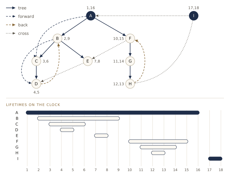
D with every edge typed. Bottom: each vertex's lifetime as an interval of the clock. Descendants' bars sit inside their ancestors' bars; a cross edge always points back to a bar that has already ended.The AssertionError branch is the case we just proved impossible. On random directed graphs it never fires, and the type counts show all four kinds occurring:
from collections import Counter

random.seed(2)
totals = Counter()
for trial in range(300):
    R = random_graph(12, random.randint(5, 40), directed=True)
    totals.update(classify(R, dfs(R)).values())
print(dict(totals))
{'tree': 2496, 'cross': 1519, 'forward': 955, 'back': 1899}
Directed acyclic graphs
A directed graph with no cycles is a directed acyclic graph, or DAG. DAGs model anything where some things must come before others: prerequisites, the steps of a build, the cells of a spreadsheet that depend on other cells, events ordered in time. The first question to ask of a directed graph is whether it has a cycle, and DFS answers it.
Theorem. A directed graph has a cycle if and only if a depth-first search of it finds a back edge.
If \((u, v)\) is a back edge, then \(v\) is an ancestor of \(u\), so the tree edges give a path from \(v\) down to \(u\), and the edge \((u, v)\) closes it into a cycle.
Conversely, suppose the graph has a cycle \(v_0 \to v_1 \to \dots \to v_k \to v_0\). The idea is to look at the cycle vertex the search reaches first. Call it \(v_i\). When \(v_i\) is discovered, every other vertex of the cycle is unvisited and reachable from \(v_i\) along the cycle, so by the lemma on explore all of them are discovered before explore(v_i) returns: they are descendants of \(v_i\). In particular the cycle vertex just before \(v_i\), which is \(v_{i-1}\) (or \(v_k\) if \(i = 0\)), is a descendant of \(v_i\) with an edge to \(v_i\). That edge is a back edge.
The first half of the proof is also an algorithm for producing the cycle: follow parent pointers from \(u\) up to \(v\).
def find_cycle(G):
    """A directed cycle of G as a list [v0, v1, ..., vk] (with an edge vk -> v0),
    or None if G is acyclic."""
    S = dfs(G)
    for u in G:
        for v in G[u]:
            if S.pre[v] <= S.pre[u] and S.post[u] <= S.post[v]:   # back edge u -> v
                path = [u]
                while path[-1] != v:
                    path.append(S.parent[path[-1]])
                return path[::-1]
    return None

print(find_cycle(D))
['B', 'C', 'D']
To test it, we compare against a slow characterization that uses no DFS theory: a graph has a cycle exactly when some edge \((u, v)\) has \(u\) reachable from \(v\). We also check that every returned cycle really is one.
def has_cycle_brute(G):
    return any(u in explore(G, v) for u in G for v in G[u])

def is_cycle(G, c):
    return all(c[(i + 1) % len(c)] in G[c[i]] for i in range(len(c)))

random.seed(8)
acyclic = agree = 0
for trial in range(400):
    R = random_graph(10, random.randint(4, 20), directed=True)
    c = find_cycle(R)
    agree += (c is not None) == has_cycle_brute(R) and (c is None or is_cycle(R, c))
    acyclic += c is None
print(f"{agree} of 400 agree ({acyclic} of the graphs were acyclic)")
400 of 400 agree (131 of the graphs were acyclic)
Topological sorting
Suppose the vertices are tasks and an edge \((u, v)\) means “\(u\) must be done before \(v\)”. A topological order (or linearization) of a directed graph is a listing of all its vertices in which every edge goes from an earlier vertex to a later one. If the graph has a cycle, no topological order exists: the first vertex of the cycle in any listing has an edge coming into it from a later one. For DAGs, DFS always finds one, and the post numbers do all the work.
Lemma. In a DAG, every edge \((u, v)\) has \(\text{post}(u) > \text{post}(v)\).
Look at the table of edge types: the only edges with \(\text{post}(u) \le \text{post}(v)\) are back edges, and a DAG has no back edges by the theorem. So listing the vertices in decreasing order of post number puts the tail of every edge before its head. We do not even need to sort: dfs already records the vertices in the order they are postvisited, and reversing that list gives decreasing post order in linear time.
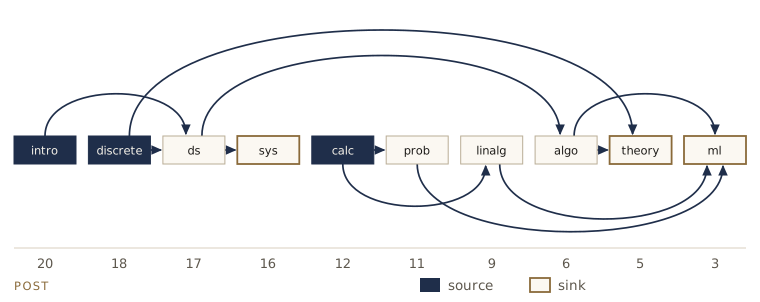
Here is a small set of course prerequisites:
prereqs = graph([("intro", "ds"), ("discrete", "ds"), ("discrete", "theory"),
                 ("ds", "algo"), ("ds", "sys"), ("algo", "theory"), ("algo", "ml"),
                 ("calc", "linalg"), ("calc", "prob"), ("linalg", "ml"),
                 ("prob", "ml")],
                directed=True)

def topological_order(G):
    """The vertices of a DAG in decreasing post order; ValueError if G has a cycle."""
    S = dfs(G)
    for u in G:
        for v in G[u]:
            if S.post[u] <= S.post[v]:
                raise ValueError(f"not a DAG: back edge {u} -> {v}")
    return S.finish[::-1]

def is_topological(G, order):
    position = {v: i for i, v in enumerate(order)}
    return (len(order) == len(G)
            and all(position[u] < position[v] for u in G for v in G[u]))

order = topological_order(prereqs)
print(order)
print(is_topological(prereqs, order))
['intro', 'discrete', 'ds', 'sys', 'calc', 'prob', 'linalg', 'algo', 'theory', 'ml']
True
On a graph with a cycle, the function refuses:
topological_order(D)
ValueError: not a DAG: back edge D -> B
Putting the pieces together: for a directed graph, having no cycle, having a topological order, and having no back edge in a depth-first search are the same property, and DFS checks it and produces the order in \(O(n + m)\) time.
Note. A DAG usually has many topological orders;
prereqshas 1,960 of them. DFS returns one of them, determined by the order in which it tries vertices and neighbors. Any of them is a correct answer.
Sources, sinks, and a second algorithm
A source is a vertex with no incoming edges, and a sink is a vertex with no outgoing edges. In prereqs the sources are calc, discrete, and intro (courses with no prerequisites) and the sinks are ml, sys, and theory (courses that are nobody’s prerequisite).
Lemma. Every DAG with at least one vertex has a source and a sink.
The vertex with the largest post number comes first in a topological order, so no edge can enter it: it is a source. The vertex with the smallest post number comes last, so no edge can leave it: it is a sink.
The existence of a source suggests another way to linearize: output a source, delete it, and repeat on what is left, which is still a DAG and so still has a source. To make this linear, keep for each vertex its number of incoming edges from vertices not yet output (its in-degree in the remaining graph), and a queue of vertices whose count has dropped to 0. Deleting a vertex decrements the counts of its out-neighbors. This is often called Kahn’s algorithm.
from collections import deque

def topological_order_by_sources(G):
    """Repeatedly output a vertex with no remaining incoming edges."""
    indegree = {v: 0 for v in G}
    for u in G:
        for v in G[u]:
            indegree[v] += 1
    ready = deque(v for v in G if indegree[v] == 0)     # the sources
    order = []
    while ready:
        u = ready.popleft()
        order.append(u)
        for v in G[u]:                                  # delete u's outgoing edges
            indegree[v] -= 1
            if indegree[v] == 0:
                ready.append(v)
    if len(order) < len(G):
        raise ValueError("not a DAG: every remaining vertex has an incoming edge")
    return order

order2 = topological_order_by_sources(prereqs)
print(order2)
print(is_topological(prereqs, order2))
['calc', 'discrete', 'intro', 'linalg', 'prob', 'ds', 'algo', 'sys', 'ml', 'theory']
True
A different order, and also valid. Each vertex enters the queue once and each edge is looked at twice (once to count, once to decrement), so this too is \(O(n + m)\). On random DAGs, both methods always produce a valid order:
def random_dag(n, m, rng=random):
    """A random DAG: shuffle the vertices, then only allow edges from earlier
    to later ones."""
    rank = list(range(n)); rng.shuffle(rank)
    edges = set()
    while len(edges) < m:
        u, v = rng.sample(range(n), 2)
        edges.add((u, v) if rank[u] < rank[v] else (v, u))
    return graph(sorted(edges), range(n), directed=True)

random.seed(4)
ok = 0
for trial in range(300):
    G = random_dag(15, random.randint(0, 40))
    ok += (is_topological(G, topological_order(G))
           and is_topological(G, topological_order_by_sources(G)))
print(ok, "of 300 random DAGs sorted correctly by both methods")
300 of 300 random DAGs sorted correctly by both methods
Strongly connected components
Connectivity in directed graphs
For undirected graphs, “connected” has an obvious meaning and DFS splits a graph into its connected components. For directed graphs we need a definition that respects direction, since a path from \(u\) to \(v\) says nothing about a path back.
Definition. Two vertices \(u\) and \(v\) of a directed graph are strongly connected if there is a path from \(u\) to \(v\) and a path from \(v\) to \(u\).
Every vertex is strongly connected to itself (by the path of length 0); the relation is symmetric by definition; and it is transitive, because paths can be joined end to end. A relation with these three properties is an equivalence relation, and it splits the vertices into disjoint classes of mutually strongly connected vertices. These classes are the strongly connected components (SCCs) of the graph. A graph with a single SCC is strongly connected.
Here is a directed graph on twelve vertices:
W = graph([("A", "B"), ("B", "C"), ("B", "D"), ("C", "A"), ("C", "F"), ("D", "E"),
           ("E", "D"), ("E", "G"), ("F", "J"), ("F", "K"), ("G", "H"), ("H", "I"),
           ("H", "J"), ("I", "J"), ("J", "G"), ("K", "L"), ("L", "K")], directed=True)
Tracing the paths by hand, \(A \to B \to C \to A\) is a cycle, so \(A, B, C\) are strongly connected; \(D\) and \(E\) point at each other; \(G \to H \to I \to J \to G\) is a cycle; \(K\) and \(L\) point at each other; and \(F\) is on no cycle, so it is a component by itself. That makes five SCCs.
Now shrink each SCC to a single vertex, and draw an edge from one SCC to another whenever some edge of the graph goes between them in that direction. The result is the meta-graph of the graph (it is also called the condensation).
Theorem. The meta-graph of any directed graph is a DAG.
If the meta-graph had a cycle through two different SCCs \(C\) and \(C'\), then every vertex of \(C\) could reach every vertex of \(C'\) and the other way round, going along the cycle. Then \(C\) and \(C'\) would be one SCC, not two.
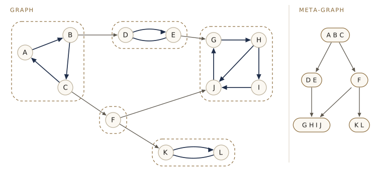
W with its five strongly connected components outlined; edges inside a component are dark, edges between components gray. Right: the meta-graph, one node per component. It is a DAG, with one source, {A, B, C}, and two sinks, {G, H, I, J} and {K, L}.So every directed graph has a two-level structure: at the top a DAG, which we already know how to handle, and inside each node of that DAG a strongly connected piece. Finding the SCCs is the first step of many algorithms on directed graphs, and it can be done in linear time.
Two facts about post numbers
The algorithm rests on two facts. The first is the lemma about explore, seen from the meta-graph.
Property 1. If
exploreis started at a vertex of a sink SCC (an SCC that is a sink of the meta-graph), it visits exactly that SCC.
From a vertex of a sink SCC, everything in the SCC is reachable, and nothing else is, because no edge leaves the SCC. For example, explore from \(K\) in W visits \(K\) and \(L\) and stops. So if we knew a vertex in a sink SCC, one call of explore would peel that SCC off. We could then continue with a sink SCC of what is left, and so on. The difficulty is finding a vertex in a sink SCC. Post numbers do not give us one directly, but they give the opposite.
Property 2. Run DFS on \(G\). If \(C\) and \(C'\) are SCCs and some edge goes from \(C\) to \(C'\), then the largest post number in \(C\) is larger than the largest post number in \(C'\).
There are two cases, depending on which component the search enters first.
- If the search reaches \(C\) first, at vertex \(x\): at that moment nothing in \(C\) or \(C'\) has been visited, and all of it is reachable from \(x\). So everything in \(C \cup C'\) is discovered, and finished, inside
explore(x). That gives \(x\) the largest post number of all of \(C \cup C'\). - If the search reaches \(C'\) first: from \(C'\) there is no path back to \(C\) (otherwise \(C\) and \(C'\) would be one SCC). So
explorefinishes all of \(C'\) without touching \(C\), and \(C\) is discovered later. Every post number in \(C\) is larger than every post number in \(C'\).
Property 2 says that ordering the SCCs by their largest post numbers, from high to low, is a topological order of the meta-graph. For a DAG, where every SCC is a single vertex, this is exactly our topological sort. In particular, the vertex with the largest post number lies in a source SCC. But what we wanted was a sink SCC.
Watch out. It is tempting to take the vertex with the smallest post number and hope it lies in a sink SCC. That is wrong in general: if the search starts in a source SCC and its first branch happens to stay inside that SCC, a vertex of the source SCC is finished before any sink is reached. Exercise 5 asks for a three-vertex example. Largest post is reliable; smallest post is not.
The algorithm
The trick is to reverse every edge. The reverse graph \(G^R\) has the same vertices as \(G\) and an edge \((v, u)\) for each edge \((u, v)\) of \(G\). Paths in \(G^R\) are paths of \(G\) read backward, so \(u\) and \(v\) are strongly connected in \(G^R\) exactly when they are in \(G\): the two graphs have the same SCCs, and the meta-graph of \(G^R\) is the meta-graph of \(G\) with its edges reversed. A source SCC of \(G^R\) is therefore a sink SCC of \(G\).
So the vertex with the largest post number in a DFS of \(G^R\) lies in a sink SCC of \(G\), which is exactly the starting point Property 1 wants. The algorithm, which is often called Kosaraju’s algorithm, is:
- Run DFS on \(G^R\) and list the vertices in decreasing order of post number.
- Run the connected-components procedure on \(G\) (DFS with a restart counter), trying the restarts in the order from step 1. Each restart visits exactly one SCC.
Our dfs accepts the restart order as a parameter, and its ccnum is the component counter, so the whole algorithm takes a few lines.
def reverse(G):
    """The reverse graph: an edge (v, u) for every edge (u, v) of G."""
    R = {v: [] for v in G}
    for u in G:
        for v in G[u]:
            R[v].append(u)
    return R

def strongly_connected_components(G):
    """The SCCs of a directed graph, sink components first (DPV section 3.4)."""
    order = dfs(reverse(G)).finish[::-1]   # step 1: decreasing post order in G^R
    S = dfs(G, order)                      # step 2: each restart peels off one SCC
    groups = {}
    for v in order:
        groups.setdefault(S.ccnum[v], []).append(v)
    return [sorted(groups[c]) for c in sorted(groups)]

print("step 1 order:", dfs(reverse(W)).finish[::-1])
for i, C in enumerate(strongly_connected_components(W), 1):
    print(f"SCC {i}: {C}")
step 1 order: ['K', 'L', 'G', 'J', 'I', 'H', 'F', 'D', 'E', 'A', 'C', 'B']
SCC 1: ['K', 'L']
SCC 2: ['G', 'H', 'I', 'J']
SCC 3: ['F']
SCC 4: ['D', 'E']
SCC 5: ['A', 'B', 'C']
Why it works, and how long it takes
Correctness. We show by induction that each restart in step 2 visits exactly one SCC, and that the SCCs are found in an order where each is a sink of the part of \(G\) not yet visited.
At the first restart, the vertex tried first has the largest post number in \(G^R\), so it lies in a source SCC of \(G^R\), which is a sink SCC of \(G\); by Property 1 the restart visits exactly that SCC. Now suppose the first \(k\) restarts have each found one SCC, and consider the next restart, at vertex \(x\) in SCC \(C\). Every vertex tried before \(x\) in the step 1 order is already visited, so \(x\) has the largest \(G^R\)-post number among unvisited vertices. By Property 2 applied to \(G^R\), any SCC with an edge into \(C\) in \(G^R\) has a larger maximum post number, so it has already been visited. Translated back to \(G\): every edge leaving \(C\) in \(G\) goes to an SCC that is already completely visited. So explore(x) visits all of \(C\) and every edge out of \(C\) leads to a visited vertex. It visits \(C\) and nothing else.
Running time. Building \(G^R\) takes one pass over the adjacency lists, \(O(n + m)\). Step 1 is a DFS, \(O(n + m)\), and it yields the order by reversing the finish list, \(O(n)\), with no sorting. Step 2 is another DFS, \(O(n + m)\). The total is linear, about three times the work of a single search.
The components of W came out in the order \(\{K, L\}\), \(\{G, H, I, J\}\), \(\{F\}\), \(\{D, E\}\), \(\{A, B, C\}\): the two sinks first, then SCCs that became sinks once those were removed, and the source last. In step 1, the search of \(G^R\) restarted at \(A\), \(D\), \(F\), \(G\), and \(K\), in that order; no vertex outside \(\{A, B, C\}\) can reach \(A\) in \(G\), so in \(G^R\) the search from \(A\) stays inside \(\{A, B, C\}\), and so on. The last restart, \(K\), finishes last and heads the order. Reading the list backward gives a topological order of the meta-graph.
Testing against the definition
The definition gives a slow but obviously correct algorithm: compute the set reachable from every vertex with one explore each, which is \(O(n(n + m))\) time, and group \(u\) with \(v\) when each reaches the other. We compare the two on random graphs, and also check the two theorems of this section: the meta-graph has no cycle, and Property 2 holds for every meta-edge.
def scc_brute(G):
    reach = {u: explore(G, u) for u in G}
    return {frozenset(v for v in G if v in reach[u] and u in reach[v]) for u in G}

def meta_graph(G, comps):
    """One vertex per SCC (numbered by position in comps), edges between them."""
    which = {v: i for i, C in enumerate(comps) for v in C}
    edges = {(which[u], which[v]) for u in G for v in G[u] if which[u] != which[v]}
    return graph(sorted(edges), range(len(comps)), directed=True)

random.seed(7)
same = dag = prop2 = strong = 0
for trial in range(300):
    n = random.randint(1, 30)
    R = random_graph(n, random.randint(0, 2 * n), directed=True)
    comps = strongly_connected_components(R)
    same += {frozenset(C) for C in comps} == scc_brute(R)
    M = meta_graph(R, comps)
    dag += find_cycle(M) is None
    post = dfs(R).post
    top = [max(post[v] for v in C) for C in comps]
    prop2 += all(top[a] > top[b] for a in M for b in M[a])
    strong += len(comps) == 1
print(f"same SCCs as brute force: {same}/300, meta-graph acyclic: {dag}/300,",
      f"property 2: {prop2}/300")
print(f"{strong} of the graphs were strongly connected")
same SCCs as brute force: 300/300, meta-graph acyclic: 300/300, property 2: 300/300
25 of the graphs were strongly connected
An application: 2SAT
A quick example of SCCs doing real work. In the 2SAT problem we are given Boolean variables and a list of clauses, each the OR of two literals (a literal is a variable \(x\) or its negation \(\bar{x}\)). We want to set each variable to true or false so that every clause has at least one true literal.
A clause \((a \lor b)\) says: if \(a\) is false then \(b\) must be true, and if \(b\) is false then \(a\) must be true. Build a directed implication graph with one vertex per literal and the two edges \(\bar{a} \to b\) and \(\bar{b} \to a\) per clause. A path from one literal to another means the first forces the second. So if \(x\) and \(\bar{x}\) lie in the same SCC, then \(x\) forces \(\bar{x}\) and \(\bar{x}\) forces \(x\), and no assignment works. The converse also holds: if no variable shares an SCC with its negation, then processing SCCs sink-first and making each literal true when its SCC is reached before its negation’s gives a satisfying assignment. (The proof is DPV exercise 3.28.) The whole test is one SCC computation, linear in the size of the formula.
def negate(lit):
    return lit[1:] if lit.startswith("~") else "~" + lit

def two_sat(clauses):
    """A satisfying assignment {variable: bool} for 2-literal clauses, or None."""
    variables = sorted({lit.lstrip("~") for clause in clauses for lit in clause})
    edges = [e for a, b in clauses for e in [(negate(a), b), (negate(b), a)]]
    G = graph(edges, [lit for x in variables for lit in (x, "~" + x)], directed=True)
    sccs = strongly_connected_components(G)          # numbered sink-first
    comp = {lit: i for i, C in enumerate(sccs) for lit in C}
    if any(comp[x] == comp["~" + x] for x in variables):
        return None
    return {x: comp[x] < comp["~" + x] for x in variables}

print(two_sat([("p", "q"), ("~p", "r"), ("~q", "~r"), ("~r", "s"), ("~s", "~p")]))
print(two_sat([("p", "q"), ("p", "~q"), ("~p", "q"), ("~p", "~q")]))
{'p': False, 'q': True, 'r': False, 's': False}
None
Check the first answer against the five clauses by hand. The second formula rules out all four combinations of values of \(p\) and \(q\), one clause each, so it has no solution. A brute-force check over all assignments of small random formulas:
def satisfies(assignment, clauses):
    def value(lit):
        return not assignment[lit[1:]] if lit.startswith("~") else assignment[lit]
    return all(value(a) or value(b) for a, b in clauses)

random.seed(6)
ok = 0
for trial in range(300):
    names = ["x1", "x2", "x3", "x4", "x5"][: random.randint(1, 5)]
    lit = lambda: random.choice(["", "~"]) + random.choice(names)
    clauses = [(lit(), lit()) for _ in range(random.randint(1, 9))]
    used = sorted({l.lstrip("~") for c in clauses for l in c})
    exists = any(satisfies(dict(zip(used, bits)), clauses)
                 for bits in product([False, True], repeat=len(used)))
    answer = two_sat(clauses)
    ok += ((answer is not None) == exists
           and (answer is None or satisfies(answer, clauses)))
print(ok, "of 300 random formulas answered correctly")
300 of 300 random formulas answered correctly
With three literals per clause the problem becomes 3SAT, which is NP-complete; we meet it in module 07. The jump from two literals to three is the jump from linear time to no known polynomial algorithm.
Depth-first search without recursion
The recursive dfs is the clearest way to write the algorithm, but as the warning earlier said, Python stops it after about a thousand nested calls. A path of 5000 vertices is enough:
chain = graph([(i, i + 1) for i in range(4999)])
print(len(chain), "vertices")
5000 vertices
dfs(chain)
RecursionError: maximum recursion depth exceeded in comparison
There are two ways out. One is to raise the limit with sys.setrecursionlimit. That works for moderate depths, but the limit exists to protect the interpreter’s own stack, and setting it very high can crash the process instead of raising a clean error. The dependable fix is to keep the stack ourselves.
The explicit stack must hold more than vertices. When the recursive version returns to a vertex, it resumes that vertex’s loop over neighbors where it left off. So each stack entry is a vertex together with an iterator over its neighbor list, which remembers the position. A vertex gets its pre number when it is pushed and its post number when its iterator runs out and it is popped, exactly as in the recursion.
def dfs_iterative(G, order=None):
    """Same results as dfs, with an explicit stack of (vertex, neighbor iterator)."""
    pre, post, parent, ccnum, finish = {}, {}, {}, {}, []
    clock = 1
    cc = 0
    for s in (G if order is None else order):
        if s in pre:
            continue
        cc += 1
        parent[s] = None
        pre[s] = clock; clock += 1; ccnum[s] = cc
        stack = [(s, iter(G[s]))]
        while stack:
            v, neighbors = stack[-1]
            for u in neighbors:                  # resume v's list where we left off
                if u not in pre:
                    parent[u] = v
                    pre[u] = clock; clock += 1; ccnum[u] = cc
                    stack.append((u, iter(G[u])))
                    break                        # go deeper first
            else:                                # v's list is used up: postvisit v
                stack.pop()
                post[v] = clock; clock += 1
                finish.append(v)
    return Search(pre, post, parent, ccnum, finish)

random.seed(9)
graphs = [random_graph(30, random.randint(0, 80), directed=random.random() < 0.5)
          for _ in range(300)]
same = all(dfs_iterative(G) == dfs(G) for G in graphs)
print("same as recursive dfs on 300 random graphs:", same)
long_chain = graph([(i, i + 1) for i in range(199_999)])
print("200,000-vertex chain, post of vertex 0:", dfs_iterative(long_chain).post[0])
same as recursive dfs on 300 random graphs: True
200,000-vertex chain, post of vertex 0: 400000
The two versions agree exactly, pre and post numbers and finishing order included, so everything built on dfs in this module can switch to dfs_iterative without change. For vertex 0 of the chain the post number is \(2n = 400{,}000\): it is the first vertex opened and the last one closed.
Watch out. A common shortcut pops a vertex, then marks all its unmarked neighbors and pushes them at once. That visits the same set of vertices, so it is fine for reachability, but it is not depth-first search: a neighbor marked early can no longer be discovered deeper in the search, so the tree it builds is different, and a vertex leaves the stack before its descendants are explored, so there is no moment at which it is “finished” and no meaningful post number. Topological sorting and the SCC algorithm need real post numbers. Exercise 6 asks for a small graph that shows the difference.
Large-scale graph exploration looks like this too. A program that crawls the web cannot recurse, and it does not know the graph in advance: it discovers vertices as it reads pages. It keeps an explicit collection of discovered but unexplored pages and a hash table of pages already seen, which plays the role of our pre dictionary. Real crawlers do not take the most recent page first; they choose the next page by a priority that estimates how useful it is. With a first-in, first-out queue instead of a stack, the same loop becomes breadth-first search, the subject of the next module.
Summary
| Problem | Algorithm | Running time |
|---|---|---|
| vertices reachable from \(s\) | explore from \(s\) |
\(O(n + m)\) |
| connected components (undirected) | DFS, one component per restart (ccnum) |
\(O(n + m)\) |
| type of every edge (directed) | DFS, then compare pre/post numbers | \(O(n + m)\) |
| does a directed graph have a cycle? | DFS, look for a back edge | \(O(n + m)\) |
| topological order of a DAG | DFS, decreasing post order (or repeatedly remove a source) | \(O(n + m)\) |
| strongly connected components | DFS on \(G^R\), then components of \(G\) in decreasing \(G^R\)-post order | \(O(n + m)\) |
| 2SAT | SCCs of the implication graph | linear in the formula |
Ideas to carry forward:
- Store graphs as adjacency lists
{u: [v, ...]}; most graph algorithms only need “the neighbors of \(u\)”, and the lists make whole-graph passes cost \(O(n + m)\). - Depth-first search is a single linear-time pass whose by-products, the forest and the pre/post numbers, answer many different questions. Intervals \([\text{pre}, \text{post}]\) are nested or disjoint, and nesting means ancestry.
- In a directed graph, only back edges go from a smaller post number to a larger one (or equal, for a self-loop). That one fact gives cycle detection, topological sorting, and, through Property 2, the SCC algorithm.
- Every directed graph is a DAG of strongly connected components. Many problems on directed graphs are solved by handling each SCC and then working along the meta-graph in topological order.
Exercises
- Run DFS by hand on the undirected graph with edges \(\{1,2\}, \{1,5\}, \{2,3\}, \{2,5\}, \{3,4\}, \{4,5\}, \{6,7\}\), trying vertices and neighbors in increasing order. Give every pre and post number, mark the tree and back edges, and list the connected components. Check your answer with
dfsandgraph. - Prove that in a depth-first search of an undirected graph every edge is a tree edge or joins a vertex to one of its ancestors; there are no cross edges. Why is there no point in distinguishing forward edges from back edges in an undirected graph? Which step of your proof fails for directed graphs?
- Show that for every vertex \(v\), \(\text{post}(v) - \text{pre}(v) + 1\) is twice the number of vertices in the subtree of the DFS forest rooted at \(v\). Use this to count the descendants of every vertex of
Win one line of Python. - Write
find_cycle_undirected(G)that returns a cycle of an undirected graph (as a list of at least three vertices) orNone, in \(O(n + m)\) time. Be careful: each tree edge appears in the child’s list pointing back to the parent, and that is not a cycle. Test it on random graphs against the fact that a graph has no cycle exactly when \(m = n - c\), where \(c\) is its number of connected components. - (a) Prove that in any DFS of a directed graph, the vertex with the largest post number lies in a source SCC. (b) Find a directed graph on three vertices and a DFS order in which the vertex with the smallest post number does not lie in a sink SCC. (c) Explain in two sentences why the SCC algorithm runs its first search on \(G^R\) rather than using smallest post numbers in \(G\).
- Consider the search that marks a vertex when it is pushed, and each time it pops a vertex pushes all of that vertex’s unmarked neighbors (marking them). Call the vertex that pushed \(v\) its parent. Find a directed graph on three vertices where these parents differ from the DFS forest of
dfs, whatever order the neighbors are pushed in, and explain why no sensible post numbers can be defined for this search. - If the graph is stored as an adjacency matrix, the loop “for each neighbor \(u\) of \(v\)” must scan a whole row. Show that DFS then takes \(\Theta(n^2)\) time on every graph, whatever \(m\) is. For which graphs is this no worse than the adjacency-list version, up to a constant factor?
- Prove that
topological_order_by_sourcesoutputs all \(n\) vertices if and only if the graph is a DAG. (For the “if” direction, use the lemma on sources. For the “only if” direction, show that when it stops early, every remaining vertex has an incoming edge from another remaining vertex, and conclude that the remaining vertices contain a cycle.) - A vertex \(v\) of a directed graph is doomed if some cycle can be reached from \(v\). Give an \(O(n + m)\) algorithm that marks all doomed vertices. (Hint: which SCCs contain a cycle? Then work along the meta-graph in reverse topological order.) Implement it with
strongly_connected_componentsandmeta_graph, and test it against a brute-force check on random graphs. - Write the implication graph of the formula \((x \lor y) \land (\bar{x} \lor z) \land (\bar{y} \lor \bar{z}) \land (\bar{x} \lor \bar{y})\), find its SCCs by hand, and read off a satisfying assignment the way
two_satdoes. Then list all satisfying assignments by brute force and check that yours is among them. - How many edges must be added to the graph
Wto make it strongly connected? Prove a lower bound in terms of the numbers of source and sink SCCs, and show that your number of edges suffices. - In your own words: explain to a classmate why depth-first search needs both pre and post numbers, giving one question that pre numbers alone cannot answer and one that post numbers answer directly.
Going further
- Dasgupta, Papadimitriou, and Vazirani, Algorithms, chapter 3 — the source for this module. Exercises 3.1–3.4 are hand runs of every algorithm here; 3.10 asks for a recursion-free
explore; 3.14 develops the source-removal sort; 3.28 proves the 2SAT reduction; 3.31 uses DFS to find biconnected components, a natural next step. - Robert Tarjan, “Depth-first search and linear graph algorithms”, SIAM Journal on Computing, 1972 — the paper that established depth-first search as a tool for linear-time graph algorithms, including a one-pass SCC algorithm that uses a single search instead of two.
- A. B. Kahn, “Topological sorting of large networks”, Communications of the ACM, 1962 — the source-removal method for topological sorting.
- Bengt Aspvall, Michael Plass, and Robert Tarjan, “A linear-time algorithm for testing the truth of certain quantified Boolean formulas”, Information Processing Letters, 1979 — the SCC algorithm for 2SAT.
- Python documentation:
graphlib, the standard library’s topological sorter, andsys.setrecursionlimit, with its warning about setting the limit too high.
These notes follow the chapters of S. Dasgupta, C. H. Papadimitriou, and U. V. Vazirani, Algorithms (McGraw-Hill, 2008), the course text. The explanations, code, figures, and exercises here are written for this course; the book remains the reference, with many more exercises.