CSE 431/531 · Module 07 · Week 6
NP-Complete Problems
Search problems, P and NP, reductions, and the chain of reductions that makes SAT, 3SAT, independent set, and friends NP-complete.
Companion reading: Dasgupta, Papadimitriou & Vazirani, Algorithms, chapter 8, “NP-complete problems”
By the end of this module you can
- Define a search problem by its efficient checking algorithm, and write the checker for SAT, TSP, or a graph problem.
- Name the hard and easy members of several look-alike pairs (2SAT and 3SAT, Euler and Rudrata, minimum and balanced cut, LP and ILP) and say what makes the easy one easy.
- State the definitions of P, NP, a reduction (the pair of polynomial-time algorithms f and h), and NP-completeness, and explain why reductions compose.
- Carry out the reductions 3SAT to independent set, SAT to 3SAT, independent set to vertex cover and clique, ZOE to subset sum, and Rudrata cycle to TSP, and prove each one correct in both directions.
- Explain the gadgets behind 3SAT to 3D matching and ZOE to Rudrata cycle, and why any problem in NP reduces to SAT through circuits.
- Recognize a pseudo-polynomial algorithm, such as the subset-sum table, and explain why it does not make an NP-complete problem easy.
- Prove a new problem NP-complete by picking a known NP-complete problem and reducing it to the new one, in the right direction.
Contents
- Search problems
- Exhaustive search
- Satisfiability
- What makes a problem a search problem
- Two easy cases of SAT
- The traveling salesman problem
- Euler and Rudrata
- Minimum cut and balanced cut
- Integer linear programming
- Three-dimensional matching
- Independent set, vertex cover, and clique
- Longest path
- Knapsack and subset sum
- NP-complete problems
- The reductions
- Unsolvable problems
- Summary
- Exercises
- Going further
For six modules we have been collecting successes. Shortest paths, minimum spanning trees, edit distance, knapsack with small capacities, independent sets in trees: each time, the space of candidate answers was exponentially large, and each time a good idea — graph search, a greedy choice, a table of subproblems — let us find the best candidate without looking at most of them. Module 06 ended with problems where that trick seemed to run out: the traveling salesman table had \(2^n\) columns.
This module is about the problems where every trick runs out. We meet a family of search problems — satisfiability of Boolean formulas, the traveling salesman problem, finding a cycle through every vertex, three-way matching, integer programming, and more — for which nobody knows an algorithm much better than trying everything. We cannot prove they are hard; that is the P versus NP question, open since the early 1970s. What we can prove is something almost as useful: they are all the same problem in different clothes. An efficient algorithm for any one of them would give efficient algorithms for all of them, and for every problem whose solutions can be checked quickly. The tool that shows this is the reduction, and most of the module is a tour of reductions.
The payoff is practical. When a problem you care about turns out to be one of these, you stop hunting for an exact polynomial-time algorithm and start choosing among the ways of coping with hardness, which is the subject of module 08.
Search problems
Exhaustive search
Almost every problem in this course has the same shape: among a huge set of candidates, find one with a given property. There are \(n!\) ways to pair \(n\) students with \(n\) projects, \(n^{n-2}\) spanning trees of the complete graph on \(n\) vertices, and in a typical graph an exponential number of paths between two vertices. Any of these problems can be solved by exhaustive search — generate the candidates one at a time and test each — but the running time is exponential, and as module 00 showed, exponential means useless beyond small inputs.
The whole art of algorithm design has been to avoid exhaustive search: to use the structure of the input to rule out almost all candidates without examining them. Greedy algorithms, dynamic programming, and network flow are the great successes. The problems in this module are the persistent failures.
Note. Faster computers do not rescue exponential algorithms; they make efficient algorithms more valuable. Suppose machines get twice as fast every two years. An algorithm that takes \(2^n\) steps can then handle one more variable every two years, about five more per decade. An \(n^2\) algorithm gains a factor of \(\sqrt{32} \approx 5.7\) in input size per decade, and an \(n \log n\) algorithm nearly a factor of 32. Exponential algorithms make slow additive progress while polynomial ones advance multiplicatively.
Satisfiability
The central problem of the module comes from logic. A Boolean variable takes the value true or false. A literal is a variable \(x\) or its negation \(\overline{x}\). A clause is an “or” of literals, such as \((x \vee \overline{y} \vee z)\), and a formula in conjunctive normal form (CNF) is an “and” of clauses, written by listing the clauses side by side:
\[(a \vee b \vee c)\;(\overline{a} \vee \overline{b})\;(\overline{a} \vee \overline{c})\;(\overline{b} \vee \overline{c}).\]A truth assignment gives every variable a value; it is satisfying if every clause contains at least one true literal. SAT (satisfiability) is the problem: given a CNF formula, find a satisfying assignment, or report that none exists. The formula above says “at least one of \(a, b, c\) is true, and no two are”, so its satisfying assignments are the three that make exactly one variable true.
In code we write a literal as a nonzero integer: variable \(i\) is i and its negation is -i, and a formula is a list of clauses, each a list of literals. (This is also the standard file format of SAT solvers.) Checking an assignment is one pass over the formula; finding one, as far as anybody knows, may require trying all \(2^n\) assignments.
from itertools import product, combinations

def variables(clauses):
    """The variables (positive integers) that occur in a formula."""
    return sorted({abs(lit) for clause in clauses for lit in clause})

def satisfies(clauses, assignment):
    """The checking algorithm for SAT: does every clause contain a true literal?"""
    return all(any(assignment[abs(lit)] == (lit > 0) for lit in clause)
               for clause in clauses)

def all_satisfying(clauses):
    """Exhaustive search: yield every satisfying assignment, trying all 2^n."""
    vs = variables(clauses)
    for values in product([False, True], repeat=len(vs)):
        assignment = dict(zip(vs, values))
        if satisfies(clauses, assignment):
            yield assignment

def brute_force_sat(clauses):
    """A satisfying assignment, or None if there is none."""
    return next(all_satisfying(clauses), None)

def show(clauses, names):
    """Pretty-print a formula; names maps variable numbers to strings."""
    lit = lambda l: ("¬" if l < 0 else "") + names[abs(l)]
    return " ".join("(" + " ∨ ".join(lit(l) for l in c) + ")" for c in clauses)

names = {1: "a", 2: "b", 3: "c", 4: "d"}
exactly_one = [[1, 2, 3], [-1, -2], [-1, -3], [-2, -3]]
print(show(exactly_one, names))
for sol in all_satisfying(exactly_one):
    print({names[v]: sol[v] for v in sol})
(a ∨ b ∨ c) (¬a ∨ ¬b) (¬a ∨ ¬c) (¬b ∨ ¬c)
{'a': False, 'b': False, 'c': True}
{'a': False, 'b': True, 'c': False}
{'a': True, 'b': False, 'c': False}
Now add three clauses that say “\(a\) implies \(b\), \(b\) implies \(c\), \(c\) implies \(a\)”. They force all three variables to be equal, which contradicts “exactly one is true”, so the new formula is unsatisfiable. The checker says so after trying all eight assignments.
all_equal = [[-1, 2], [-2, 3], [-3, 1]]
contradiction = exactly_one + all_equal
print(show(contradiction, names))
print(brute_force_sat(contradiction))
(a ∨ b ∨ c) (¬a ∨ ¬b) (¬a ∨ ¬c) (¬b ∨ ¬c) (¬a ∨ b) (¬b ∨ c) (¬c ∨ a)
None
What makes a problem a search problem
SAT has a property that will define the whole class of problems in this module: a proposed solution is easy to check, even when it is hard to find. Checking needs two things. The solution must be short, no longer than a polynomial in the size of the input, so that we can read it. And there must be a fast algorithm that decides whether it really is a solution.
Definition. A search problem is given by an algorithm \(C\) that takes an instance \(I\) and a proposed solution \(S\) and runs in time polynomial in \(\lvert I \rvert\), the length of \(I\). We say \(S\) is a solution of \(I\) exactly when \(C(I, S)\) returns true. Solving the search problem means: given \(I\), find some \(S\) with \(C(I, S) =\) true, or report that there is none.
The instance is the input data (here, a formula), and \(C\) is the checking algorithm (here, satisfies, which runs in time linear in the length of the formula). Because \(C\) runs in polynomial time, it cannot even read a solution longer than a polynomial in \(\lvert I \rvert\), so short solutions come for free with the definition.
Two easy cases of SAT
Nobody knows a polynomial-time algorithm for SAT; the best algorithms known are exponential in the worst case. But two restricted versions are easy, for quite different reasons:
- A Horn formula has at most one positive literal in each clause. The greedy algorithm of module 05 starts with every variable false and sets a variable true only when some implication forces it; it finds a satisfying assignment or proves there is none in linear time.
- In 2SAT every clause has at most two literals. A clause \((x \vee y)\) is the pair of implications \(\overline{x} \Rightarrow y\) and \(\overline{y} \Rightarrow x\); drawing these as a directed graph on the \(2n\) literals, the formula is satisfiable exactly when no variable lies in the same strongly connected component as its negation. The algorithm of module 03 finds the components in linear time.
Allow three literals per clause and the problem, called 3SAT, is as hard as SAT itself; we prove this later in the module. (In these notes a 3SAT formula is one whose clauses have at most three literals.) The step from two to three is typical of this subject: a small change in the rules moves a problem from easy to, apparently, hopeless.
The traveling salesman problem
In the traveling salesman problem (TSP) we are given \(n\) cities, the distance \(d_{ij}\) between every pair, and a budget \(b\). We must find a tour — a cycle that visits every city exactly once — of total length at most \(b\), or report that there is none. In other words, we want an ordering \(\tau(1), \dots, \tau(n)\) of the cities with
\[d_{\tau(1)\tau(2)} + d_{\tau(2)\tau(3)} + \dots + d_{\tau(n)\tau(1)} \le b.\]We usually think of TSP as an optimization problem: find the shortest tour. Why add a budget? Because the definition of a search problem requires that solutions be checkable, and “this tour is shortest” is not a property anybody knows how to check quickly. “This is a tour of length at most \(b\)” is:
def check_tour(dist, budget, tour):
    """The checking algorithm for TSP: is `tour` an ordering of all cities
    whose closed length is at most the budget?"""
    n = len(dist)
    if sorted(tour) != list(range(n)):
        return False
    length = sum(dist[tour[i]][tour[(i + 1) % n]] for i in range(n))
    return length <= budget

dist = [[0, 3, 4, 2, 7],
        [3, 0, 4, 6, 3],
        [4, 4, 0, 5, 8],
        [2, 6, 5, 0, 6],
        [7, 3, 8, 6, 0]]
print(check_tour(dist, 20, [0, 1, 4, 3, 2]))   # 3 + 3 + 6 + 5 + 4 = 21
print(check_tour(dist, 20, [0, 2, 1, 4, 3]))   # 4 + 4 + 3 + 6 + 2 = 19
print(check_tour(dist, 20, [0, 2, 1, 4]))      # misses city 3
False
True
False
The budget costs nothing in difficulty. If we can solve the optimization version, we solve the search version by comparing the optimum with \(b\). Conversely, a search algorithm finds the optimum by binary search on the budget: the optimal length is an integer between 0 and the sum of all distances, so \(O(\log \sum d_{ij})\) calls suffice, and that is polynomial in the number of bits of the input (exercise 1). Phrasing optimization problems as search problems lets us compare them with true search problems such as SAT in a single framework.
Nobody knows a polynomial algorithm for TSP. Exhaustive search tries \((n-1)!\) tours, and the dynamic program of module 06 takes \(O(n^2 2^n)\) time: much better, still exponential. Compare the minimum spanning tree problem, which in search form asks for a spanning tree of total weight at most \(b\) and is solved greedily in module 05. A tour minus one edge is a spanning tree that is not allowed to branch. That one restriction seems to be the difference between easy and hard.
Euler and Rudrata
An Euler path in a graph is a path that uses every edge exactly once (vertices may repeat). Euler’s theorem gives a complete answer: a graph with at least one edge has an Euler path if and only if the part of it with edges is connected and at most two vertices have odd degree. (If there are two, the path must start at one and end at the other.) The proof is constructive, and it gives a polynomial-time algorithm for the search problem Euler path.
A Rudrata cycle uses every vertex exactly once and returns to its start; a Rudrata path does the same without returning. The classic instance is the knight’s tour: the vertices are the 64 squares of a chessboard and the edges join squares a knight’s move apart. These are usually called Hamiltonian cycles and paths; we use the name Rudrata, after the ninth-century Kashmiri poet who posed the knight’s-tour question. The search problem Rudrata cycle asks for such a cycle or a report that none exists. It looks like TSP with all distances equal, and indeed no polynomial algorithm is known.
The Euler and Rudrata problems differ in two ways: edges versus vertices, and path versus cycle. The second difference turns out to be cosmetic — we reduce one Rudrata version to the other later in the module — so it is “every edge once” versus “every vertex once” that separates easy from hard.
Minimum cut and balanced cut
A cut is a set of edges whose removal disconnects the graph. Minimum cut asks, given a graph and a budget \(b\), for a cut with at most \(b\) edges. It is easy: give each edge capacity 1 and compute a maximum flow from a fixed vertex \(s\) to each of the other \(n-1\) vertices; by the max-flow min-cut theorem (DPV chapter 7) the smallest of these flows is the size of the smallest cut. The randomized contraction algorithm in module 05 is another way.
Often the smallest cut just chops off one low-degree vertex, which is not very informative. Balanced cut asks for a partition of the vertices into \(S\) and \(T\) with \(\lvert S \rvert, \lvert T \rvert \ge n/3\) and at most \(b\) edges between them. Balanced cuts are what we want for clustering — for instance, splitting a graph of similar neighboring pixels into large coherent regions of an image — and the balance requirement makes the problem hard.
Integer linear programming
A linear program asks for real numbers \(x_1, \dots, x_n\) that satisfy a set of linear inequalities \(Ax \le b\) and maximize a linear objective. Linear programming is covered in DPV chapter 7, which is not part of this course; the one fact we need is that it can be solved in polynomial time. Integer linear programming (ILP) asks for a nonnegative integer vector \(x\) with \(Ax \le b\), or a report that none exists. (An objective \(c \cdot x \ge g\) is one more inequality, so the search version needs no separate objective.) Requiring integers changes everything: no polynomial algorithm for ILP is known.
A clean special case is zero-one equations (ZOE): given an \(m \times n\) matrix \(A\) whose entries are 0 or 1, find a vector \(x \in \{0, 1\}^n\) with \(Ax = \mathbf{1}\), where \(\mathbf{1}\) is the all-ones vector. In words: choose a set of columns that together contain exactly one 1 in every row.
Three-dimensional matching
In bipartite matching we have \(n\) items on each of two sides and a list of compatible pairs, and we want \(n\) disjoint pairs; it is solvable in polynomial time by maximum flow (DPV chapter 7). 3D matching adds a third side. There are three disjoint sets \(X\), \(Y\), \(Z\) of \(n\) elements each — think of people, tasks, and time slots — and a list of compatible triples \((x, y, z)\). We want \(n\) triples that use every element exactly once. No polynomial algorithm is known.
Independent set, vertex cover, and clique
Three problems about a graph \(G = (V, E)\):
- Independent set: given \(G\) and a goal \(g\), find \(g\) vertices no two of which are adjacent. In module 06 we solved it on trees in linear time; on general graphs no polynomial algorithm is known.
- Vertex cover: given \(G\) and a budget \(b\), find \(b\) vertices that touch every edge. It is a special case of set cover from module 05: the universe is \(E\), and each vertex contributes the set of edges it touches.
- Clique: given \(G\) and a goal \(g\), find \(g\) vertices every two of which are adjacent.
Longest path
Shortest paths are easy (module 04). In longest path we are given a graph with nonnegative edge weights, two vertices \(s\) and \(t\), and a goal \(g\), and we want a simple path (no repeated vertices) from \(s\) to \(t\) of weight at least \(g\). Without the word “simple” the problem would be silly, since a path could go around a cycle forever. With it, no efficient algorithm is known; notice that with unit weights and \(g = n-1\) it asks for a Rudrata path from \(s\) to \(t\).
Knapsack and subset sum
In knapsack, as in module 06, there are \(n\) items with integer weights \(w_i\) and values \(v_i\), a capacity \(W\), and (for the search version) a goal \(g\); we want items of total weight at most \(W\) and total value at least \(g\). The dynamic program runs in \(O(nW)\) time. That looks polynomial, but it is not: the input writes \(W\) in about \(\log W\) bits, and \(W\) is exponential in \(\log W\).
Definition. An algorithm is pseudo-polynomial if its running time is polynomial in the input length and the numeric values in the input, but not necessarily in the input length alone.
If the numbers were written in unary — twelve as 111111111111 — the \(O(nW)\) algorithm would be polynomial in the (now much longer) input. So unary knapsack is in the easy column, while knapsack with numbers in binary is not known to be.
A special case strips knapsack to the bone. In subset sum we are given integers \(a_1, \dots, a_n\) and a target \(t\), and want a subset that adds up to exactly \(t\). (It is knapsack with \(v_i = w_i\) and \(g = W = t\).) The same table idea solves it: keep the set of sums reachable with the first \(i\) numbers.
def subset_sum(numbers, target):
    """Dynamic programming over reachable sums.  Returns (subset or None, steps),
    where steps counts inner-loop iterations: about n * target."""
    parent = [None] * (target + 1)   # parent[s]: index of the number that reached s
    parent[0] = -1
    steps = 0
    for i, a in enumerate(numbers):
        for s in range(target, a - 1, -1):   # downward: each number used at most once
            steps += 1
            if parent[s] is None and parent[s - a] is not None:
                parent[s] = i
    if parent[target] is None:
        return None, steps
    chosen, s = [], target
    while s > 0:                             # walk back through the parents
        i = parent[s]
        chosen.append(numbers[i])
        s -= numbers[i]
    return chosen, steps

numbers = [27, 41, 16, 58, 33, 9]
print(subset_sum(numbers, 100))
print(subset_sum(numbers, 101))
print(subset_sum(numbers, 102))
([9, 33, 58], 422)
([58, 16, 27], 428)
(None, 434)
The target 102 is not a sum of any subset, and the table says so; a no-answer costs about as much as a yes-answer, since every round scans the table either way. When parent[s] is set to i during round i, the sum s - a was reachable using only numbers before i (the downward loop has not yet touched smaller sums in this round), so the walk back uses each number at most once. The table has \(t + 1\) entries and each of the \(n\) rounds scans at most all of them once: \(O(nt)\) time. (The step counts are a little below \(nt = 600\) because round \(i\) scans only the sums from \(a_i\) up.)
Now make the numbers bigger without making the instance any more interesting: multiply every number and the target by \(10^k\). The answers do not change. Each step of \(k\) adds about 3.3 bits to each number, while the work grows by a factor of about 10.
for k in range(4):
    scaled = [a * 10 ** k for a in numbers]
    target = 100 * 10 ** k
    bits = sum(a.bit_length() for a in scaled) + target.bit_length()
    subset, steps = subset_sum(scaled, target)
    print(f"k = {k}   input bits = {bits:3d}   steps = {steps:9,d}")
k = 0   input bits =  39   steps =       422
k = 1   input bits =  62   steps =     4,166
k = 2   input bits =  85   steps =    41,606
k = 3   input bits = 108   steps =   416,006
The input grows linearly while the work grows exponentially. With 30-digit numbers the table would have \(10^{30}\) entries. So subset sum is only easy when its numbers are small, and in general it is one of the hard problems.
Watch out. “\(O(nW)\)” and “\(O(nt)\)” hide the trap in the letter: \(W\) is a value, not a length. Always ask how the running time compares with the number of bits needed to write the input. An algorithm that is polynomial in the numbers is exponential in their length.
NP-complete problems
Hard problems, easy problems
Here are the problems of the last section side by side. Each hard problem on the left has an easy relative on the right.
| Hard (NP-complete) | Easy (in P) | Why the easy one is easy |
|---|---|---|
| 3SAT | 2SAT, Horn SAT | strongly connected components; greedy |
| TSP | minimum spanning tree | greedy |
| longest path | shortest path | Dijkstra, Bellman–Ford |
| 3D matching | bipartite matching | maximum flow |
| knapsack | unary knapsack | dynamic programming |
| independent set | independent set on trees | dynamic programming |
| integer linear programming | linear programming | polynomial LP algorithms |
| Rudrata path | Euler path | Euler’s degree condition |
| balanced cut | minimum cut | maximum flow |
The right column is diverse: each problem is easy for its own reason, found with its own technique. The left column is the opposite. The problems there are all hard for the same reason: as we will show, each of them can be translated into any other. They are one problem in nine disguises.
P and NP
With the definition of a search problem in hand, two classes are easy to state.
Definition. NP is the class of all search problems. P is the class of search problems that can be solved in polynomial time: there is an algorithm that, given any instance \(I\), runs in time polynomial in \(\lvert I \rvert\) and either returns a solution or correctly reports that none exists.
Every problem in the table is in NP (write the checker for each; they are all short). Every problem in the right column is in P. And P is contained in NP by definition: its members are search problems that happen to be solvable quickly. The big question is whether the containment is strict:
\[\text{Is } \mathbf{P} \ne \mathbf{NP}\text{?}\]That is, is there a search problem whose solutions are easy to check but hard to find? Most researchers believe so. One reason is the accumulated failure to find fast algorithms for problems like SAT and TSP despite enormous effort. Another is a thought experiment: a formal mathematical proof can be checked line by line by a program, so “find a proof of this statement of at most a given length” is a search problem. If P were equal to NP, finding proofs would be about as easy as checking them, which would be astonishing. Yet nobody has been able to prove P \(\ne\) NP; it is one of the central open problems of mathematics.
Note. The letters: P is for polynomial, and NP is for nondeterministic polynomial time. A nondeterministic algorithm is an imaginary machine that may guess at each step and is credited with success if some sequence of guesses succeeds; a search problem is exactly one whose solutions such a machine can guess and then verify in polynomial time. Most textbooks also define NP as a class of decision problems, questions with a yes-or-no answer such as “is this formula satisfiable?”, rather than search problems. The two views give the same theory; the search view is closer to what an algorithm designer wants.
Reductions
Even granting P \(\ne\) NP, why should these particular problems be hard? The evidence is a web of reductions, translations of one problem into another.
Definition. A reduction from search problem \(A\) to search problem \(B\) is a pair of polynomial-time algorithms: \(f\) transforms any instance \(I\) of \(A\) into an instance \(f(I)\) of \(B\), and \(h\) transforms any solution \(S\) of \(f(I)\) into a solution \(h(S)\) of \(I\). In addition, if \(f(I)\) has no solution, then \(I\) has no solution. We write \(A \to B\).
A reduction turns any algorithm for \(B\) into an algorithm for \(A\): apply \(f\), run the algorithm for \(B\), and either apply \(h\) to its solution or report that there is none. If the algorithm for \(B\) runs in polynomial time, so does the whole thing, because \(f(I)\) was produced in polynomial time and so has length polynomial in \(\lvert I \rvert\), and a polynomial of a polynomial is a polynomial.
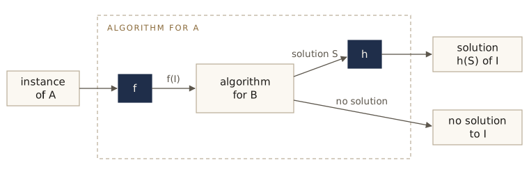
Proving a reduction correct always takes the same three steps:
- \(f\) and \(h\) run in polynomial time.
- If \(S\) is a solution of \(f(I)\), then \(h(S)\) is a solution of \(I\).
- If \(f(I)\) has no solution, then \(I\) has none. This is usually proved as its contrapositive: if \(I\) has a solution, then so does \(f(I)\).
Forgetting step 3 is the most common mistake. Without it, a transformation that always produces an unsolvable instance would “reduce” anything to anything.
Two uses of a reduction. Up to now we used reductions to solve problems: we knew how to do \(B\) (say, shortest paths) and reduced \(A\) to it. In this module we use them the other way round. If \(A\) is believed to be hard and \(A \to B\), then \(B\) must be at least as hard, since a fast algorithm for \(B\) would give one for \(A\). Efficient algorithms flow backward along the arrow; hardness flows forward.
Watch out. To show that a new problem \(B\) is hard, reduce a known hard problem to \(B\), not \(B\) to it. Reducing \(B\) to SAT only shows that \(B\) is no harder than SAT, which is true of every problem in NP, easy ones included.
Reductions compose. If \(A \to B\) by \((f_{AB}, h_{AB})\) and \(B \to C\) by \((f_{BC}, h_{BC})\), then \(A \to C\) by \((f_{BC} \circ f_{AB},\; h_{AB} \circ h_{BC})\): transform the instance twice, then map the solution back twice. Each composite runs in polynomial time because the intermediate objects have polynomial length, and the “no solution” condition passes through both stages. So the relation “reduces to” is transitive, and a chain of reductions is a reduction.
NP-completeness
Definition. A search problem \(B\) is NP-complete if \(B\) is in NP and every search problem in NP reduces to \(B\).
This is a demanding property: an NP-complete problem can express every search problem there is. It is remarkable that such problems exist at all. But they do, and every problem in the left column of the table is one. Two consequences make the definition useful:
- If some NP-complete problem is in P, then every problem in NP reduces to a problem in P, so P \(=\) NP. Turned around: if P \(\ne\) NP, as almost everyone believes, then no NP-complete problem has a polynomial algorithm. The picture is of P at the easy bottom of NP and the NP-complete problems at the hard top.
- To show a new problem \(B\) in NP is NP-complete, it is enough to reduce one known NP-complete problem \(A\) to it. Every problem in NP reduces to \(A\), and by transitivity to \(B\).
The second point is how NP-completeness proofs work in practice, and how the rest of this module is organized. We need one problem proved NP-complete from scratch — SAT, via circuits, at the end of the module — and then a tree of reductions carries the property to all the others.
Factoring
The first hard problem in the course was factoring: given an integer, find its prime factors (module 01). It is in NP (multiply the factors back and check each is prime). No polynomial algorithm is known, and the security of RSA rests on that. Yet factoring is not believed to be NP-complete. One difference: every integer has a prime factorization, so the definition of factoring never needs the clause “or report that none exists”, which the NP-complete problems use essentially. Another: factoring can be solved in polynomial time on a quantum computer (DPV chapter 10), while no such algorithm is known for SAT or TSP. Factoring seems to sit strictly between P and the NP-complete problems.
The reductions
Here is the plan. We show that every problem in NP reduces to SAT, and that SAT reduces, directly or through a chain, to each of the other problems. Together these make all of them NP-complete.
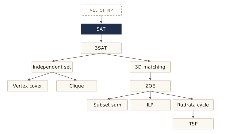
Warm-up: Rudrata path to Rudrata cycle
In Rudrata \((s,t)\)-path we are given a graph \(G\) and two vertices \(s\) and \(t\), and want a path from \(s\) to \(t\) that visits every vertex exactly once. Could Rudrata cycle be easier? No.
Construction. Let \(G'\) be \(G\) plus one new vertex \(x\) and two new edges \(\{s, x\}\) and \(\{x, t\}\).
Solutions map back. The new vertex \(x\) has only two neighbors, so any Rudrata cycle of \(G'\) passes through \(s, x, t\) consecutively. Deleting \(x\) and its two edges leaves a path from \(s\) to \(t\) through every other vertex exactly once: a Rudrata \((s,t)\)-path of \(G\). That deletion is \(h\).
No solution maps to no solution. Contrapositive: if \(G\) has a Rudrata \((s,t)\)-path, add the edges \(\{t, x\}\) and \(\{x, s\}\) to close it into a Rudrata cycle of \(G'\).
Running time. \(f\) adds one vertex and two edges; \(h\) deletes them. Both take linear time.
A reduction in the opposite direction also exists (exercise 6), so the two versions are equivalent. That one was a near-identity. The reductions that follow connect problems that look nothing alike.
3SAT to independent set
One is about Boolean formulas, the other about graphs. How can a graph express logic?
The idea. A satisfying assignment makes at least one literal true in every clause. So satisfying a formula amounts to picking one literal from each clause to be the true one, subject to consistency: we must never pick \(x\) in one clause and \(\overline{x}\) in another. Conversely, any consistent choice of one literal per clause gives a satisfying assignment (set the chosen literals true, and any unmentioned variable arbitrarily). Picking “one per group, with some pairs forbidden” is what an independent set does.
Construction of \(f\), for a formula with \(m\) clauses:
- For each clause, make one vertex per literal in it, and join all the clause’s vertices to each other: a triangle for a three-literal clause, an edge for a two-literal clause, a lone vertex for a one-literal clause. An independent set can then take at most one vertex per clause.
- Join every pair of vertices, in any clauses, whose literals are opposite, like \(x\) and \(\overline{x}\). An independent set can then never choose both.
- Set the goal \(g = m\), so the independent set must take exactly one vertex from each clause.
Let’s build it for a formula of our own with four variables and four clauses:
\[(a \vee \overline{b} \vee c)\;(\overline{a} \vee b \vee d)\;(b \vee \overline{c} \vee \overline{d})\;(\overline{a} \vee \overline{b}).\]A vertex is a pair (clause index, position), and label records its literal. We use a dictionary of adjacency lists for graphs, as in earlier modules.
def sat_to_independent_set(clauses):
    """f: the graph (adjacency lists), the goal g, and each vertex's literal."""
    label = {(i, j): lit
             for i, clause in enumerate(clauses) for j, lit in enumerate(clause)}
    graph = {v: [] for v in label}
    for u, v in combinations(label, 2):
        same_clause = u[0] == v[0]
        opposite = label[u] == -label[v]
        if same_clause or opposite:
            graph[u].append(v)
            graph[v].append(u)
    return graph, len(clauses), label

F = [[1, -2, 3], [-1, 2, 4], [2, -3, -4], [-1, -2]]
G, g, label = sat_to_independent_set(F)
edges = sum(len(nbrs) for nbrs in G.values()) // 2
print(show(F, names))
print(f"{len(G)} vertices, {edges} edges, goal g = {g}")
(a ∨ ¬b ∨ c) (¬a ∨ b ∨ d) (b ∨ ¬c ∨ ¬d) (¬a ∨ ¬b)
11 vertices, 18 edges, goal g = 4
Ten edges come from the clauses (three triangles and one edge) and eight join opposite literals. Now solve the independent set instance by brute force — try every set of \(g\) vertices — and map the answer back with \(h\): set each chosen literal true.
def is_independent(graph, S):
    S = set(S)
    return all(v not in S for u in S for v in graph[u])

def find_independent_set(graph, g):
    """Exhaustive search over all g-subsets of the vertices."""
    for S in combinations(graph, g):
        if is_independent(graph, S):
            return set(S)
    return None

def independent_set_to_assignment(S, label, clauses):
    """h: make every chosen literal true; unconstrained variables get False."""
    assignment = {x: False for x in variables(clauses)}
    for v in S:
        assignment[abs(label[v])] = label[v] > 0
    return assignment

S = find_independent_set(G, g)
print("independent set:", sorted(S))
print("chosen literals:", show([[label[v]] for v in sorted(S)], names))
A = independent_set_to_assignment(S, label, F)
print({names[x]: A[x] for x in A}, "satisfies F:", satisfies(F, A))
independent set: [(0, 0), (1, 2), (2, 1), (3, 1)]
chosen literals: (a) (d) (¬c) (¬b)
{'a': True, 'b': False, 'c': False, 'd': True} satisfies F: True
The search picked \(a\) from the first clause, \(d\) from the second, \(\overline{c}\) from the third, and \(\overline{b}\) from the fourth. Making those four literals true gives the assignment \(a = d =\) true, \(b = c =\) false, and the checker confirms that it satisfies the formula.
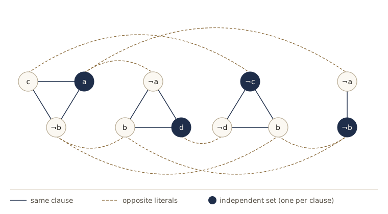
Now the proof that this works for every formula.
Solutions map back. Let \(S\) be an independent set of size \(g = m\). The vertices of each clause are pairwise adjacent, so \(S\) has at most one vertex per clause; with \(m\) vertices and \(m\) clauses it has exactly one. No two vertices of \(S\) carry opposite literals, since those are adjacent, so setting every literal of \(S\) true is consistent. It makes one literal in every clause true: the assignment \(h(S)\) satisfies the formula.
No solution maps to no solution. Contrapositive: suppose the formula has a satisfying assignment. In each clause pick one true literal and take its vertex. That is \(m\) vertices. Two of them in the same clause? No, we picked one per clause. Two with opposite literals? No, both are true under the same assignment. So they form an independent set of size \(g\).
Running time. The graph has one vertex per literal occurrence, at most \(3m\), and we examine every pair: \(O(m^2)\) time for \(f\). \(h\) reads off \(S\) in linear time.
What about unsatisfiable formulas? The contradiction formula from earlier has seven clauses and fifteen literal occurrences; its graph has no independent set of size 7. And on random small formulas, the two problems always agree:
import random

def random_formula(n_vars, n_clauses):
    """Clauses of 1 to 3 distinct variables, each negated with probability 1/2."""
    formula = []
    for _ in range(n_clauses):
        vs = random.sample(range(1, n_vars + 1), random.randint(1, 3))
        formula.append([v if random.random() < 0.5 else -v for v in vs])
    return formula

G2, g2, _ = sat_to_independent_set(contradiction)
print("contradiction:", len(G2), "vertices, independent set of size", g2, "->",
      find_independent_set(G2, g2))

random.seed(531)
agree, n_sat = 0, 0
for trial in range(60):
    phi = random_formula(3, random.randint(4, 6))
    G3, g3, lab3 = sat_to_independent_set(phi)
    S3 = find_independent_set(G3, g3)
    sat = brute_force_sat(phi) is not None
    n_sat += sat
    if S3 is None:
        agree += not sat
    else:
        agree += satisfies(phi, independent_set_to_assignment(S3, lab3, phi))
print(f"{agree} of 60 random formulas agree ({n_sat} satisfiable, {60 - n_sat} not)")
contradiction: 15 vertices, independent set of size 7 -> None
60 of 60 random formulas agree (42 satisfiable, 18 not)
The reduction also works for clauses of any length, so it is really a reduction from SAT; we state it for 3SAT because that keeps the graph small and because the tree needs only 3SAT.
SAT to 3SAT
Here SAT is reduced to a restricted version of SAT. The point is that the restriction to three literals per clause does not make SAT any easier.
Construction. Keep every clause with at most three literals. Replace each clause \((a_1 \vee a_2 \vee \dots \vee a_k)\) with \(k > 3\) (the \(a_i\) are literals) by a chain of \(k - 2\) clauses, using \(k - 3\) new variables \(y_1, \dots, y_{k-3}\):
\[(a_1 \vee a_2 \vee y_1)\;(\overline{y_1} \vee a_3 \vee y_2)\;(\overline{y_2} \vee a_4 \vee y_3)\;\cdots\;(\overline{y_{k-3}} \vee a_{k-1} \vee a_k).\]Read \(y_i\) as “the true literal is further along the chain”. The first clause says: \(a_1\) or \(a_2\) is true, or pass the obligation on. Each middle clause says: if the obligation was passed to me, either my \(a\) is true or I pass it on. The last clause says: if the obligation reaches the end, \(a_{k-1}\) or \(a_k\) must be true.
Lemma. For every assignment to \(a_1, \dots, a_k\): the clause \((a_1 \vee \dots \vee a_k)\) is satisfied if and only if some setting of \(y_1, \dots, y_{k-3}\) satisfies all the chain clauses.
Proof. Suppose the chain is satisfied but every \(a_i\) is false. The first clause forces \(y_1\) true; then the second forces \(y_2\) true; and so on, until \(y_{k-3}\) is true and the last clause has no true literal — a contradiction. So some \(a_i\) is true. Conversely, suppose \(a_i\) is true. Set \(y_1, \dots, y_{i-2}\) true and the remaining \(y\)’s false. Clauses before the one containing \(a_i\) are satisfied by their positive \(y\), the clause containing \(a_i\) is satisfied by it, and clauses after it are satisfied by their \(\overline{y}\), whose \(y\) is false.
Applying the lemma to each long clause separately (their \(y\)’s are distinct): the new formula is satisfiable if and only if the old one is. Two formulas related this way are called equisatisfiable. The map \(h\) is to forget the \(y\)’s: a satisfying assignment of the new formula, restricted to the original variables, satisfies the original formula. The construction adds \(k - 3\) variables and \(k - 3\) clauses per long clause, so the new formula is at most a constant times longer, and \(f\) runs in linear time.
def sat_to_3sat(clauses):
    """f: split each clause of more than three literals into a chain of clauses."""
    fresh = max(variables(clauses)) + 1
    result = []
    for clause in clauses:
        k = len(clause)
        if k <= 3:
            result.append(list(clause))
            continue
        ys = list(range(fresh, fresh + k - 3))
        fresh += k - 3
        result.append([clause[0], clause[1], ys[0]])
        for i in range(1, k - 3):
            result.append([-ys[i - 1], clause[i + 1], ys[i]])
        result.append([-ys[-1], clause[-2], clause[-1]])
    return result

long_names = {1: "a", 2: "b", 3: "c", 4: "d", 5: "e", 6: "f",
              7: "y1", 8: "y2", 9: "y3"}
wide = [[1, -2, 3, 4, -5, 6]]
print(show(wide, long_names))
print(show(sat_to_3sat(wide), long_names))
(a ∨ ¬b ∨ c ∨ d ∨ ¬e ∨ f)
(a ∨ ¬b ∨ y1) (¬y1 ∨ c ∨ y2) (¬y2 ∨ d ∨ y3) (¬y3 ∨ ¬e ∨ f)
A randomized check on formulas with long clauses: the original and transformed formulas are equisatisfiable, and restricting a solution of the new one always satisfies the old one.
def random_long_formula(n_vars, n_clauses):
    formula = []
    for _ in range(n_clauses):
        vs = random.sample(range(1, n_vars + 1), random.randint(1, n_vars))
        formula.append([v if random.random() < 0.5 else -v for v in vs])
    return formula

random.seed(8)
ok, n_sat, longest = 0, 0, 0
for trial in range(200):
    phi = random_long_formula(5, random.randint(3, 8))
    psi = sat_to_3sat(phi)
    assert all(len(c) <= 3 for c in psi)
    longest = max(longest, len(variables(psi)))
    sol = brute_force_sat(psi)
    original_sat = brute_force_sat(phi) is not None
    n_sat += original_sat
    if sol is None:
        ok += not original_sat
    else:
        ok += satisfies(phi, {x: sol[x] for x in variables(phi)})
print(f"{ok} of 200 agree ({n_sat} satisfiable); "
      f"up to {longest} variables after splitting")
200 of 200 agree (182 satisfiable); up to 15 variables after splitting
A further restriction. For the 3D matching reduction later we need 3SAT to stay hard even when each variable occurs in at most three clauses, with each literal at most twice. Another rewriting achieves this. If variable \(x\) occurs \(k \ge 3\) times, replace its occurrences by \(k\) new variables \(x_1, \dots, x_k\), one per occurrence, and add the cycle of implications
\[(\overline{x_1} \vee x_2)\;(\overline{x_2} \vee x_3)\;\cdots\;(\overline{x_{k-1}} \vee x_k)\;(\overline{x_k} \vee x_1).\]These say \(x_1 \Rightarrow x_2 \Rightarrow \dots \Rightarrow x_k \Rightarrow x_1\), so in any satisfying assignment all the copies are equal and act as the single variable \(x\) (exercise 4). Each copy now occurs three times — once where \(x\) was, once positively and once negatively in the cycle — so each of its literals occurs at most twice. Variables that occurred at most twice already satisfy both limits.
Independent set to vertex cover and clique
Some reductions are ingenious; these two record that one problem is a thin disguise of another.
Lemma. For a graph \(G = (V, E)\) and a set \(S \subseteq V\), the following are equivalent: (1) \(S\) is an independent set of \(G\); (2) \(V - S\) is a vertex cover of \(G\); (3) \(S\) is a clique of the complement \(\overline{G}\), the graph on \(V\) whose edges are exactly the pairs that are not edges of \(G\).
Proof. \(S\) is independent exactly when no edge has both ends in \(S\), that is, when every edge has at least one end in \(V - S\), which says \(V - S\) is a vertex cover. And no pair in \(S\) is an edge of \(G\) exactly when every pair in \(S\) is an edge of \(\overline{G}\).
Independent set to vertex cover. \(f\) maps \((G, g)\) to \((G, \lvert V \rvert - g)\); \(h\) maps a vertex cover \(C\) to \(V - C\). If \(G\) has no vertex cover of size \(\lvert V \rvert - g\), it has no independent set of size \(g\), since the complement of one would be the other. Both maps take linear time.
Independent set to clique. \(f\) maps \((G, g)\) to \((\overline{G}, g)\) and \(h\) is the identity. Building \(\overline{G}\) takes \(O(\lvert V \rvert^2)\) time.
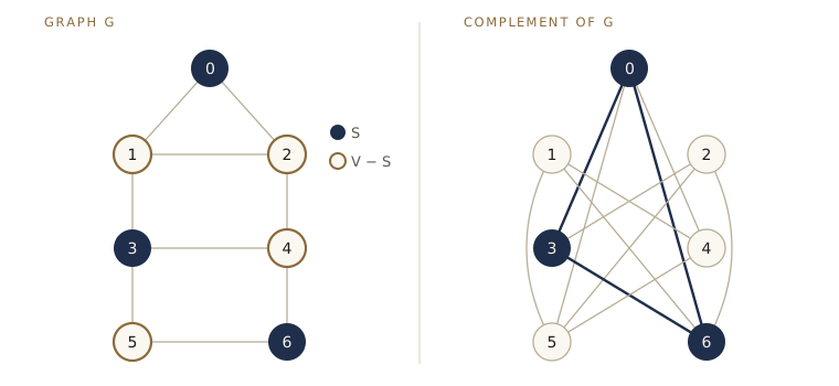
The lemma is easy to check exhaustively on small graphs: for every graph and every subset, the three properties agree.
def is_vertex_cover(graph, C):
    C = set(C)
    return all(u in C or v in C for u in graph for v in graph[u])

def is_clique(graph, S):
    return all(v in graph[u] for u, v in combinations(S, 2))

def complement(graph):
    return {u: [v for v in graph if v != u and v not in graph[u]] for u in graph}

def random_graph(n, p):
    graph = {u: [] for u in range(n)}
    for u, v in combinations(range(n), 2):
        if random.random() < p:
            graph[u].append(v)
            graph[v].append(u)
    return graph

random.seed(7)
checked = 0
for trial in range(100):
    G4 = random_graph(7, 0.4)
    H4 = complement(G4)
    for r in range(8):
        for S in combinations(G4, r):
            rest = set(G4) - set(S)
            assert (is_independent(G4, S) == is_vertex_cover(G4, rest)
                    == is_clique(H4, S))
            checked += 1
print(f"checked {checked:,} (graph, subset) pairs")

example = {0: [1, 2], 1: [0, 2, 3], 2: [0, 1, 4], 3: [1, 4, 5],
           4: [2, 3, 6], 5: [3, 6], 6: [4, 5]}
best = max((S for r in range(8) for S in combinations(example, r)
            if is_independent(example, S)), key=len)
print("largest independent set:", best)
print("vertex cover:", sorted(set(example) - set(best)))
print("clique in complement:", is_clique(complement(example), best))
checked 12,800 (graph, subset) pairs
largest independent set: (0, 3, 6)
vertex cover: [1, 2, 4, 5]
clique in complement: True
3SAT to 3D matching
Now two problems that look entirely different: a formula, and a set of triples in which we must cover every element exactly once. We sketch the reduction; the idea is to build gadgets, small pieces of the target instance that imitate variables and clauses.
Variable gadget. For each variable \(x\), create two elements \(b_0, b_1\) of the first set, two elements \(c_0, c_1\) of the second, and four elements \(p_0, p_1, p_2, p_3\) of the third, with four triples arranged in a ring:
\[(b_0, c_1, p_0),\quad (b_1, c_0, p_2),\quad (b_0, c_0, p_1),\quad (b_1, c_1, p_3).\]The elements \(b_0, b_1, c_0, c_1\) appear in no other triples. To cover them, a matching must use either the first two triples or the last two: if \(b_0\) takes \((b_0, c_1, p_0)\), then \(c_1\) is used and \(b_1\) must take \((b_1, c_0, p_2)\); if \(b_0\) takes \((b_0, c_0, p_1)\), then \(c_0\) is used and \(b_1\) must take \((b_1, c_1, p_3)\). So the gadget has exactly two states. Call the first state \(x =\) true: it uses \(p_0\) and \(p_2\) and leaves \(p_1\) and \(p_3\) free. The second state, \(x =\) false, uses \(p_1, p_3\) and frees \(p_0, p_2\).
Clause gadget. For each clause, create one new element in each of the first two sets, say \(b_c\) and \(c_c\), and one triple per literal of the clause: for a literal \(x\), the triple \((b_c, c_c, p)\) with \(p\) one of \(p_1, p_3\) of \(x\)’s gadget (free exactly when \(x\) is true); for a literal \(\overline{x}\), with \(p\) one of \(p_0, p_2\) (free exactly when \(x\) is false). The pair \(b_c, c_c\) can be covered only through a free third element, that is, through a literal that is true. Each literal occurrence gets its own \(p\); there are enough because, by the restricted 3SAT above, each literal occurs at most twice.
Padding. With \(n\) variables and \(m\) clauses there are \(4n\) third-set elements; the variable gadgets use \(2n\) and the clauses \(m\), leaving \(2n - m\) uncovered. (This is positive: each variable occurs at most three times, and we may assume each clause has at least two literals, since a one-literal clause forces the value of its variable, which can be substituted into the formula beforehand (repeatedly, if that creates new one-literal clauses); so \(2m \le 3n < 4n\).) Add \(2n - m\) extra pairs of first- and second-set elements, each forming a triple with every third-set element, to absorb whatever is left over. Now each of the three sets has exactly \(4n\) elements.
Why it works, and the time. From a matching, read each variable’s value off its gadget’s state; every clause pair is covered through a free element, so every clause has a true literal. From a satisfying assignment, set the gadgets accordingly, cover each clause through one of its true literals, and let the padding take the rest. The instance has \(O(n + m)\) elements and \(O((n + m)^2)\) triples (the padding dominates), so \(f\) is polynomial, and \(h\) reads off the \(n\) gadget states.
3D matching to ZOE
Zero-one equations are a general-purpose language for combinatorial constraints, and 3D matching translates into it directly.
Construction. Given \(q\) elements in each of the three sets and \(k\) triples, make one 0–1 variable \(x_j\) per triple (\(x_j = 1\) means “triple \(j\) is chosen”), and one equation per element: the sum of \(x_j\) over the triples containing that element equals 1. The matrix \(A\) has \(3q\) rows and \(k\) columns, and column \(j\) has 1s in the three rows of triple \(j\)’s elements.
Why it works. A 0–1 vector \(x\) with \(Ax = \mathbf{1}\) chooses a set of triples that covers every element exactly once, which is precisely a 3D matching, and vice versa; \(h\) reads off the triples with \(x_j = 1\). Building \(A\) takes \(O(qk)\) time.
Here is a small instance of our own: people Ana and Ben, tasks grading and lab, days Mon and Tue, and five compatible triples.
people, tasks, days = ["Ana", "Ben"], ["grading", "lab"], ["Mon", "Tue"]
triples = [("Ana", "grading", "Mon"), ("Ana", "lab", "Tue"), ("Ben", "lab", "Mon"),
           ("Ben", "grading", "Tue"), ("Ben", "lab", "Tue")]

def matching_to_zoe(elements, triples):
    """f: one row per element, one column per triple;
    A[r][j] = 1 if triple j contains element r."""
    return [[1 if e in t else 0 for t in triples] for e in elements]

A = matching_to_zoe(people + tasks + days, triples)
for element, row in zip(people + tasks + days, A):
    print(f"{element:>8}  {row}")
     Ana  [1, 1, 0, 0, 0]
     Ben  [0, 0, 1, 1, 1]
 grading  [1, 0, 0, 1, 0]
     lab  [0, 1, 1, 0, 1]
     Mon  [1, 0, 1, 0, 0]
     Tue  [0, 1, 0, 1, 1]
Each column has three 1s, one for each element of its triple, and each row is an equation. The row for Ben, for instance, says that exactly one of the last three triples is chosen.
ZOE to subset sum
ZOE has many equations with 0–1 coefficients; subset sum has one equation with large coefficients. The bridge is an old idea: a vector of digits is a number.
Construction. We want a set of columns of \(A\) whose sum is the all-ones vector. Read each column, top to bottom, as the digits of an integer, and the all-ones vector as the digits of the target. Then a set of columns summing to \(\mathbf{1}\) gives a set of integers summing to the target.
The converse is the delicate part: integers can add up to the target through carries even though the digit vectors do not add up to \(\mathbf{1}\). In base 2, the column digits \(0101 + 0110 + 0100\) (that is, \(5 + 6 + 4\)) add to \(1111 = 15\) even though the second digit position receives three 1s and the first receives none. The fix is to use base \(k + 1\), where \(k\) is the number of columns. At most \(k\) digits, each 0 or 1, are ever added in one position, so no position reaches \(k + 1\), no carry occurs, and integers sum to the target exactly when digit vectors sum to \(\mathbf{1}\).
def zoe_to_subset_sum(A, base):
    """f: column j becomes the integer whose digits are A[0][j], A[1][j], ..."""
    m, k = len(A), len(A[0])
    numbers = [sum(A[r][j] * base ** (m - 1 - r) for r in range(m)) for j in range(k)]
    target = sum(base ** (m - 1 - r) for r in range(m))
    return numbers, target

def zoe_solutions(A):
    """Exhaustive search: all column sets whose sum is the all-ones vector."""
    k = len(A[0])
    return [S for r in range(k + 1) for S in combinations(range(k), r)
            if all(sum(row[j] for j in S) == 1 for row in A)]

def subset_sum_solutions(numbers, target):
    k = len(numbers)
    return [S for r in range(k + 1) for S in combinations(range(k), r)
            if sum(numbers[j] for j in S) == target]

Z = [[1, 0, 1, 0, 0],
     [0, 1, 1, 1, 1],
     [0, 1, 0, 0, 0],
     [1, 0, 1, 1, 0]]
print("ZOE solutions:      ", zoe_solutions(Z))
for base in [2, len(Z[0]) + 1]:
    nums, t = zoe_to_subset_sum(Z, base)
    print(f"base {base}: numbers {nums}, target {t}",
          "-> subsets", subset_sum_solutions(nums, t))
ZOE solutions:       [(0, 1)]
base 2: numbers [9, 6, 13, 5, 4], target 15 -> subsets [(0, 1), (1, 3, 4)]
base 6: numbers [217, 42, 253, 37, 36], target 259 -> subsets [(0, 1)]
In base 2, the reduction invents a false solution: columns 1, 3, and 4 (numbering from 0) give \(6 + 5 + 4 = 15\), although their digits add to 0 in the top row and to 3 in the second row. In base 6 the solutions match exactly. The numbers have \(m\) digits in base \(k + 1\), so about \(m \log_2(k + 1)\) bits each: \(f\) runs in polynomial time. And \(h\) is the identity on sets of column indices.
The composition of our last two reductions is a reduction from 3D matching to subset sum. We can run it end to end and solve the result with the dynamic program from the first section:
nums, t = zoe_to_subset_sum(A, len(triples) + 1)
chosen, steps = subset_sum(nums, t)
print("numbers:", nums, " target:", t)
print("steps:", steps)
print("matching:", [triples[nums.index(x)] for x in chosen])
numbers: [7998, 7813, 1338, 1513, 1333]  target: 9331
steps: 26665
matching: [('Ben', 'lab', 'Tue'), ('Ana', 'grading', 'Mon')]
It finds the only matching — Ana grades on Monday, Ben runs the lab on Tuesday. (Reading triples back with nums.index works here because the five numbers are distinct.) The dynamic program was fast because the instance is tiny. In general the target has \(3q\) digits in base \(k+1\), so the table has more than \((k+1)^{3q - 1}\) entries: exponential, exactly as the warning about pseudo-polynomial time predicted.
ZOE to ILP
Some reductions need no cleverness at all: if \(A\) is a special case of \(B\) — its instances are among \(B\)’s instances, with the same solutions — then \(A \to B\) with \(f\) and \(h\) both the identity. For example, 3SAT is a special case of SAT, so 3SAT \(\to\) SAT trivially. This gives the cheapest NP-completeness proofs: a problem that generalizes an NP-complete problem is NP-complete (provided it is in NP). Set cover, for instance, generalizes vertex cover, so it is NP-complete.
ZOE is a special case of ILP after a small rewriting. ILP wants a nonnegative integer \(x\) with \(Ax \le b\). Write each equation \(\sum_j a_{ij} x_j = 1\) as two inequalities, \(\sum_j a_{ij} x_j \le 1\) and \(-\sum_j a_{ij} x_j \le -1\), and add \(x_j \le 1\) for every \(j\). A nonnegative integer vector satisfying all of these is a 0–1 vector with \(Ax = \mathbf{1}\), and conversely. The rewriting doubles the rows and adds \(k\) more: linear time.
ZOE to Rudrata cycle
This reduction goes through an intermediate problem. In Rudrata cycle with paired edges, we are given a graph, possibly with several parallel edges between the same two vertices, and a set \(C\) of pairs of edges; we want a Rudrata cycle that, for every pair \((e, e')\) in \(C\), uses exactly one of \(e\) and \(e'\).
ZOE to Rudrata cycle with paired edges. Given \(Ax = \mathbf{1}\) with \(m\) equations and \(k\) variables, build a single big cycle made of \(m + k\) “bundles” of parallel edges between consecutive vertices:
- for each variable \(x_j\), a bundle of two parallel edges, one meaning \(x_j = 1\) and one meaning \(x_j = 0\);
- for each equation, a bundle with one parallel edge for each variable that appears in it.
A Rudrata cycle must go around, crossing each bundle on exactly one of its edges. So it chooses a value for every variable and one variable for every equation. The pairs in \(C\) tie the two choices together: for each equation and each variable \(x_j\) in it, pair the edge “\(x_j\) in this equation” with the edge “\(x_j = 0\)”. If \(x_j = 1\), the edge \(x_j = 0\) is unused, so every equation containing \(x_j\) must choose \(x_j\); if \(x_j = 0\), no equation may choose \(x_j\). Since each equation chooses exactly one variable, and must choose every variable of value 1 in it, each equation has exactly one variable equal to 1. That is a solution of \(Ax = \mathbf{1}\), and the argument runs backward too. The graph has \(m + k\) vertices and \(O(mk)\) edges and pairs.
Getting rid of the pairs. A gadget does the pairing inside an ordinary graph. It is a ladder-like subgraph of 12 new vertices that attaches to the rest of the graph only at four corner vertices \(a, b\) (on one side) and \(c, d\) (on the other), replacing a paired couple of edges \(\{a, b\}\) and \(\{c, d\}\). Its rungs contain vertices of degree 2, which a Rudrata cycle must pass through the moment it reaches a neighbor, and checking the few possible routes shows that any Rudrata cycle of the whole graph crosses the gadget in exactly one of two ways: it enters at \(a\), visits all 12 internal vertices, and leaves at \(b\); or it enters at \(c\), visits them all, and leaves at \(d\). So the gadget behaves exactly like the two edges \(\{a, b\}\) and \(\{c, d\}\) with the constraint “exactly one of them is used”. Replace each pair in \(C\) by a gadget. If an edge \(\{a, b\}\) belongs to several pairs, then once its first gadget is in place, the gadget’s edge from corner \(a\) to its first internal vertex is used exactly when the cycle crosses from \(a\) to \(b\), so that edge takes the place of \(\{a, b\}\) in the remaining pairs. Each replacement adds 12 vertices, so the final graph has polynomial size, and its Rudrata cycles correspond one-to-one to the paired-edge Rudrata cycles of the original. The details are in DPV section 8.3.
Rudrata cycle to TSP
Construction. Given a graph \(G\) on \(n\) vertices, make a TSP instance with the same \(n\) cities: the distance between \(u\) and \(v\) is 1 if \(\{u, v\}\) is an edge of \(G\) and \(1 + \alpha\) otherwise, for a constant \(\alpha > 0\) of our choosing. The budget is \(n\).
Why it works. A tour has \(n\) legs, each of length at least 1, so it fits the budget \(n\) exactly when every leg has length 1, that is, when every leg is an edge of \(G\) — when the tour is a Rudrata cycle of \(G\). So \(h\) is the identity, and if \(G\) has no Rudrata cycle, every tour uses at least one long leg and costs at least \(n + \alpha\). Building the distance matrix takes \(O(n^2)\) time.
from itertools import permutations

def tsp_from_graph(graph, alpha):
    """f: distance 1 along edges of the graph, 1 + alpha between non-neighbors."""
    n = len(graph)
    return [[0 if u == v else (1 if v in graph[u] else 1 + alpha) for v in range(n)]
            for u in range(n)]

def shortest_tour_length(dist):
    """Exhaustive search over the (n-1)! tours that start at city 0."""
    n = len(dist)
    return min(sum(dist[t[i]][t[(i + 1) % n]] for i in range(n))
               for t in ([0] + list(p) for p in permutations(range(1, n))))

def has_rudrata_cycle(graph):
    n = len(graph)
    return any(all(t[(i + 1) % n] in graph[t[i]] for i in range(n))
               for t in ([0] + list(p) for p in permutations(range(1, n))))

random.seed(42)
graphs = [random_graph(6, 0.5) for trial in range(40)]
for alpha in [1, 10]:
    counts = {True: 0, False: 0}
    for G5 in graphs:
        best = shortest_tour_length(tsp_from_graph(G5, alpha))
        rudrata = has_rudrata_cycle(G5)
        assert rudrata == (best <= 6) and (rudrata or best >= 6 + alpha)
        counts[rudrata] += 1
    print(f"alpha = {alpha:2d}: {counts[True]} graphs with a Rudrata cycle (tour 6), "
          f"{counts[False]} without (tour >= {6 + alpha})")
alpha =  1: 14 graphs with a Rudrata cycle (tour 6), 26 without (tour >= 7)
alpha = 10: 14 graphs with a Rudrata cycle (tour 6), 26 without (tour >= 16)
The free parameter \(\alpha\) gives two useful variants, both important in module 08:
- With \(\alpha = 1\) every distance is 1 or 2, and such distances satisfy the triangle inequality \(d_{ik} \le d_{ij} + d_{jk}\) (the right side is at least 2, the left at most 2). So TSP stays NP-complete even for distances that obey the triangle inequality — the version for which good approximation algorithms exist.
- With \(\alpha\) huge, the instance has a gap: either the best tour costs \(n\), or every tour costs at least \(n + \alpha\). An algorithm guaranteed to find a tour within a factor \(c\) of the optimum, run on an instance with \(\alpha > (c - 1)n\), would tell the two cases apart and so solve Rudrata cycle. Unless P \(=\) NP, general TSP cannot be approximated at all.
Any problem in NP to SAT
We have reduced SAT to everything in the tree. To close the circle we show that every problem in NP reduces to SAT. This is the Cook–Levin theorem, proved independently by Stephen Cook and Leonid Levin in the early 1970s, and it is what makes SAT the root of the tree. We go through a more flexible version of SAT.
Circuit SAT. A Boolean circuit is a directed acyclic graph whose vertices are gates: AND and OR gates with two incoming edges, NOT gates with one, known inputs labeled true or false, and unknown inputs labeled “?”. One sink is the output. Given values for the unknown inputs, we evaluate the gates in topological order and read the output. Circuit SAT asks for values of the unknown inputs that make the output true, or a report that there are none.
SAT is a special case: a CNF formula is a circuit with an OR gate tree for each clause, NOT gates on negated variables, and an AND gate tree joining the clauses. The other direction, Circuit SAT \(\to\) SAT, gives each gate \(g\) a variable of its own and writes clauses that force \(g\) to have the right value given its inputs:
| Gate | Clauses | What they say |
|---|---|---|
| \(g\) = true | \((g)\) | \(g\) is true |
| \(g\) = false | \((\overline{g})\) | \(g\) is false |
| \(g = \text{NOT } h\) | \((g \vee h)\;(\overline{g} \vee \overline{h})\) | exactly one of \(g, h\) is true |
| \(g = h_1 \text{ AND } h_2\) | \((\overline{g} \vee h_1)\;(\overline{g} \vee h_2)\;(g \vee \overline{h_1} \vee \overline{h_2})\) | \(g\) implies both inputs; both inputs imply \(g\) |
| \(g = h_1 \text{ OR } h_2\) | \((g \vee \overline{h_1})\;(g \vee \overline{h_2})\;(\overline{g} \vee h_1 \vee h_2)\) | each input implies \(g\); \(g\) implies some input |
Finally add the clause \((g_{\text{out}})\) for the output gate. A satisfying assignment of these clauses must give every gate the value the circuit computes from the unknown inputs, and must make the output true, so the satisfying assignments correspond one-to-one to the input settings that satisfy the circuit; \(h\) reads off the input variables. There are at most three clauses per gate: linear time. Let’s test it on a small circuit of our own that computes \((p \vee (\text{true} \wedge q)) \wedge \neg(q \wedge r)\).
circuit = [                      # (name, kind, inputs...) in topological order
    ("p", "input"), ("q", "input"), ("r", "input"), ("one", "true"),
    ("g1", "and", "one", "q"),
    ("g2", "or", "p", "g1"),
    ("g3", "and", "q", "r"),
    ("g4", "not", "g3"),
    ("out", "and", "g2", "g4"),
]

def evaluate(circuit, inputs):
    value = {}
    for name, kind, *args in circuit:
        if kind == "input":  value[name] = inputs[name]
        elif kind == "true": value[name] = True
        elif kind == "false": value[name] = False
        elif kind == "not":  value[name] = not value[args[0]]
        elif kind == "and":  value[name] = value[args[0]] and value[args[1]]
        elif kind == "or":   value[name] = value[args[0]] or value[args[1]]
    return value

def circuit_to_sat(circuit, output):
    """f: one variable per gate, the clauses of the table, and the clause (output)."""
    var = {gate[0]: i + 1 for i, gate in enumerate(circuit)}
    clauses = []
    for name, kind, *args in circuit:
        g = var[name]
        h = [var[a] for a in args]
        if kind == "true":    clauses += [[g]]
        elif kind == "false": clauses += [[-g]]
        elif kind == "not":   clauses += [[g, h[0]], [-g, -h[0]]]
        elif kind == "and":   clauses += [[-g, h[0]], [-g, h[1]], [g, -h[0], -h[1]]]
        elif kind == "or":    clauses += [[g, -h[0]], [g, -h[1]], [-g, h[0], h[1]]]
    return clauses + [[var[output]]], var

inputs = ["p", "q", "r"]
from_circuit = {vals for vals in product([False, True], repeat=3)
                if evaluate(circuit, dict(zip(inputs, vals)))["out"]}
cnf, var = circuit_to_sat(circuit, "out")
from_cnf = [tuple(a[var[x]] for x in inputs) for a in all_satisfying(cnf)]
print(len(cnf), "clauses over", len(var), "variables")
print("circuit is satisfied by", len(from_circuit), "input settings;",
      "the CNF has", len(from_cnf), "satisfying assignments")
print("same input settings:", set(from_cnf) == from_circuit)
16 clauses over 9 variables
circuit is satisfied by 4 input settings; the CNF has 4 satisfying assignments
same input settings: True
Every problem in NP reduces to Circuit SAT. Let \(A\) be any search problem, with checking algorithm \(C(I, S)\) running in polynomial time. We know nothing else about \(A\), and we need nothing else. The key fact, from DPV section 7.7, is that any algorithm running in polynomial time on inputs of a fixed length can be written out as a Boolean circuit of polynomial size. The idea: a computer is a circuit that updates its memory once per clock tick, and an algorithm that runs for \(T\) steps on \(T\) bits of memory can be unrolled into \(T\) layers of copies of that circuit, polynomial in total when \(T\) is. So, given an instance \(I\):
- Build the circuit for \(C\) on inputs of length \(\lvert I \rvert + \ell\), where \(\ell\) bounds the solution length (polynomial in \(\lvert I \rvert\)).
- Make the first \(\lvert I \rvert\) inputs known, set to the bits of \(I\), and leave the other \(\ell\) inputs unknown.
The output is true exactly when the unknown inputs spell a solution \(S\) of \(I\). So satisfying assignments of this circuit are solutions of \(I\) (\(h\) reads them off), and if \(I\) has no solution the circuit is unsatisfiable. Composing with Circuit SAT \(\to\) SAT:
Theorem. Every search problem in NP reduces to SAT. Together with the reductions above, SAT, 3SAT, independent set, vertex cover, clique, 3D matching, ZOE, subset sum, ILP, Rudrata cycle and path, and TSP are all NP-complete.
Knapsack generalizes subset sum and longest path generalizes Rudrata path, so they are NP-complete too; balanced cut is also NP-complete, by a longer reduction we omit.
Unsolvable problems
NP-complete problems are hard, but they can be solved: exhaustive search always works, given enough time. Some well-defined problems cannot be solved by any algorithm at all, however slow. They are called unsolvable (or undecidable).
The first was found by Alan Turing in 1936, before there were computers to run programs on. In modern terms: given a program and an input, will the program stop? Suppose some function terminates(program, data) always answered this correctly. Then we could write:
def terminates(program, data):
    """Suppose this returned True exactly when program(data) eventually stops."""
    raise NotImplementedError("no such function can exist")

def paradox(program):
    if terminates(program, program):
        while True:        # loop forever
            pass
    # otherwise stop at once
What does paradox(paradox) do? If terminates(paradox, paradox) is true, it loops forever, so the answer was wrong. If it is false, it stops immediately, so the answer was wrong again. Either way terminates fails on this input, so no correct terminates can exist. This is the halting problem.
Note. Unsolvability spreads by reduction just as NP-completeness does. For example, “does this program ever reach this line?” is unsolvable, because a solution would answer the halting problem (ask about the line after the program’s last statement). Unsolvable problems are not only about programs: whether a polynomial equation with integer coefficients, in several variables, has an integer solution is also unsolvable, a result completed in 1970.
Summary
| Problem | Search version | Status | How we know |
|---|---|---|---|
| SAT | satisfying assignment of a CNF formula | NP-complete | every problem in NP → Circuit SAT → SAT |
| 3SAT | the same, clauses of at most 3 literals | NP-complete | SAT → 3SAT (chain clauses) |
| independent set | \(g\) pairwise non-adjacent vertices | NP-complete | 3SAT → independent set (triangles) |
| vertex cover, clique | \(b\) vertices touching every edge; \(g\) pairwise adjacent vertices | NP-complete | complement set; complement graph |
| 3D matching | \(n\) disjoint triples covering everything | NP-complete | 3SAT → 3D matching (gadgets) |
| ZOE, ILP | 0–1 solution of \(Ax = \mathbf{1}\); integer solution of \(Ax \le b\) | NP-complete | 3D matching → ZOE → ILP |
| subset sum, knapsack | subset with sum \(t\); items within weight and value bounds | NP-complete; \(O(nt)\) pseudo-polynomial | ZOE → subset sum (base \(k+1\)) |
| Rudrata cycle, TSP | cycle through every vertex; tour within budget | NP-complete | ZOE → Rudrata cycle → TSP |
| 2SAT, Horn SAT, MST, shortest path, Euler path, min cut, LP, bipartite matching | — | in P | the techniques of modules 03–06 and DPV chapter 7 |
Ideas to carry forward:
- A search problem is defined by a fast checker. NP is the class of search problems; P is the part we can solve in polynomial time. Whether P \(=\) NP is open.
- A reduction \(A \to B\) is a pair \((f, h)\) of polynomial-time maps, correct in both directions. Algorithms flow from \(B\) back to \(A\); hardness flows from \(A\) forward to \(B\). To prove \(B\) NP-complete, reduce a known NP-complete problem to \(B\).
- Reductions are built from gadgets: small pieces of the target instance that imitate the choices (variables) and constraints (clauses) of the source.
- NP-completeness is a verdict about the worst case over all instances, and it tells you to stop looking for a fast exact algorithm. Module 08 is about what to do instead.
Exercises
- Suppose you have a polynomial-time algorithm for the search version of TSP (tour within budget \(b\)). Show how to find the length of the shortest tour with \(O(\log D)\) calls, where \(D\) is the sum of all distances, and then how to find a shortest tour itself. Explain why the total time is polynomial in the input length.
- Suppose
sat_decide(clauses)answers only yes or no. Show how to find a satisfying assignment with at most \(n + 1\) calls, by fixing the variables one at a time. Implement it withbrute_force_sat(...) is not Nonestanding in forsat_decide, and test it on the formulas of this module. - Write checking algorithms, with their running times, for 3D matching, vertex cover, and longest path. For longest path, what exactly must the checker verify about the proposed path?
- Prove that in any satisfying assignment of the implication cycle \((\overline{x_1} \vee x_2)(\overline{x_2} \vee x_3)\cdots(\overline{x_k} \vee x_1)\) all the \(x_i\) are equal. Then prove that replacing a variable’s \(k \ge 3\) occurrences by copies joined in this way preserves satisfiability, and count the variables and clauses of the new formula.
- A classmate argues: “2SAT is NP-complete, because every 2SAT formula is a 3SAT formula, so 2SAT reduces to 3SAT.” Find the flaw. What would a correct NP-completeness proof for 2SAT have to show, and why do we not expect one?
- Reduce Rudrata cycle to Rudrata \((s,t)\)-path. (Hint: pick a vertex \(v\), split it into two copies that share its neighbors, and attach a new vertex of degree 1 to each copy.) Prove both directions.
- Implement a reduction from Rudrata cycle to SAT. Use variables \(x_{v,i}\) meaning “vertex \(v\) is in position \(i\) of the cycle”, and write clauses saying that every position holds exactly one vertex, every vertex has exactly one position, and consecutive positions (including the last and the first) hold adjacent vertices. Test it against
has_rudrata_cycleon random graphs with 5 vertices. How many variables and clauses does a graph on \(n\) vertices produce? - Dense subgraph: given a graph and integers \(a\) and \(b\), find \(a\) vertices with at least \(b\) edges among them. Prove that it is NP-complete by showing it generalizes one of the problems of this module.
- Prove that
subset_sumruns in \(O(nt)\) time. Then show that subset sum restricted to instances whose numbers are all at most \(n^3\) is in P. Why does this not contradict the NP-completeness of subset sum? - In the ZOE to subset sum reduction, prove that base \(k + 1\) never produces a carry. The base-2 example in the module shows that a small base can invent false solutions. What is the smallest base, as a function of the number of columns \(k\), for which the reduction is correct on every matrix? Prove that it works, and give a matrix on which the next smaller base fails.
- Check the gate clauses of the Circuit SAT table by writing out truth tables. Then add an XOR gate (\(g\) is true exactly when one of \(h_1, h_2\) is true) to
circuit_to_satusing four clauses, and test it by comparing satisfying inputs as in the module. - In your own words: explain to a friend who has taken data structures why “we proved problem X is NP-complete” is useful news for a programmer, what it does not mean (give at least two things it does not rule out), and why the direction of the reduction matters.
Going further
- Dasgupta, Papadimitriou, and Vazirani, Algorithms, chapter 8 — the source for this module. Exercises 8.1–8.2 (optimization, search, and decision), 8.4 (a subtly wrong NP-completeness proof), 8.10 (NP-completeness by generalization), 8.14, 8.19, and 8.20 are good practice.
- Stephen A. Cook, “The complexity of theorem-proving procedures”, STOC 1971 — the paper that introduced NP-completeness and proved it for satisfiability.
- Richard M. Karp, “Reducibility among combinatorial problems”, 1972 — twenty-one problems, many from this module, shown NP-complete by a tree of reductions.
- Michael R. Garey and David S. Johnson, Computers and Intractability: A Guide to the Theory of NP-Completeness (W. H. Freeman, 1979) — the classic catalog of NP-complete problems and reduction techniques.
- P versus NP problem and the list of NP-complete problems on Wikipedia.
These notes follow the chapters of S. Dasgupta, C. H. Papadimitriou, and U. V. Vazirani, Algorithms (McGraw-Hill, 2008), the course text. The explanations, code, figures, and exercises here are written for this course; the book remains the reference, with many more exercises.