CSE 431/531 · Module 05 · Week 4
Greedy Algorithms
Minimum spanning trees and the cut property, Kruskal and Prim, union–find, Huffman codes, Horn formulas, and set cover.
Companion reading: Dasgupta, Papadimitriou & Vazirani, Algorithms, chapter 5, “Greedy algorithms”
By the end of this module you can
- State the cut property, prove it with an exchange argument, and use it to show that Kruskal’s and Prim’s algorithms return minimum spanning trees.
- Implement a disjoint-sets (union–find) structure with union by rank and path compression, and explain the \(O(\log n)\) worst-case and \(O(\log^* n)\) amortized bounds.
- Run Kruskal’s and Prim’s algorithms by hand and in code, and give their running times.
- Build a Huffman code for a set of frequencies, prove that merging the two least frequent symbols is optimal, and compare its cost with the entropy.
- Decide whether a Horn formula is satisfiable with the “stingy” greedy algorithm, prove it correct, and implement it in linear time.
- Apply the greedy algorithm for set cover, prove that it is within a factor \(\ln n\) of optimal, and give an instance on which it is not optimal.
- Recognize the two usual shapes of a greedy correctness proof — an exchange argument and an invariant — and say which one a given algorithm needs.
Contents
- Greedy choices, and when they fail
- Minimum spanning trees
- Huffman encoding
- Horn formulas
- Set cover
- Summary
- Exercises
- Going further
In module 04 we met Dijkstra’s algorithm. It grows a set of vertices whose distances are known, and at every step it adds the vertex that is currently closest to the source. It never reconsiders a choice, and yet the distances it reports are exact. That style of algorithm has a name, and this module is about it.
A greedy algorithm builds a solution one piece at a time. At each step it takes the piece that looks best right now according to a simple local rule, and it never undoes a choice. Greedy algorithms are short and fast. The hard part is knowing when they are right, and much of this module is about the arguments that tell us so.
We look at four problems. For minimum spanning trees, Huffman codes, and Horn formulas, a well-chosen greedy rule gives an optimal answer, and we prove it. For set cover, the natural greedy rule is not optimal, but we can prove it is never far off, which is a first taste of the approximation algorithms in module 08. Along the way we build the union–find data structure, one of the most useful small data structures in all of computing.
Greedy choices, and when they fail
Before the successes, a failure, so that we take nothing for granted. Suppose you must pay an amount using as few coins as possible. The greedy rule is obvious: use the largest coin that fits, and repeat.
def greedy_change(amount, coins):
    """Pay `amount` by repeatedly using the largest coin that still fits."""
    used = []
    for c in sorted(coins, reverse=True):
        while amount >= c:
            amount -= c
            used.append(c)
    return used

print(greedy_change(68, [1, 5, 10, 25]))   # US coins: greedy is optimal here
print(greedy_change(6, [1, 3, 4]))         # but 3 + 3 uses only two coins
[25, 25, 10, 5, 1, 1, 1]
[4, 1, 1]
With US coins the greedy answer happens to be optimal. With coins of value 1, 3, and 4, it pays 6 as \(4 + 1 + 1\) when \(3 + 3\) is better: taking the 4 looked best at the moment but left an awkward remainder. (Dynamic programming, in module 06, solves the coin problem for any set of coins.) So a greedy rule needs a proof, and the proof has to explain why an early choice can never paint us into a corner.
Note. Correctness proofs for greedy algorithms nearly always take one of two shapes. An exchange argument takes an optimal solution that disagrees with the greedy choice and modifies it, without making it worse, until it agrees; so some optimal solution contains the greedy choice. An invariant argument shows that everything the algorithm has committed to so far is forced, or safe, in every good solution. The cut property and Huffman’s algorithm use exchanges; the Horn-formula algorithm uses an invariant.
Minimum spanning trees
The problem
Suppose a campus wants to connect seven buildings, labeled a to g, with cable. Cable can only run along certain routes, and each route has a cost, in thousands of dollars. Every building must be able to reach every other one, directly or through other buildings. What is the cheapest set of routes to lay?
This is a graph problem. The buildings are vertices, the possible routes are undirected edges, and each edge \(e\) has a weight \(w_e\), its cost. We store an undirected weighted graph in two ways, both used throughout the module: as an edge list of triples (u, v, w), and as a dict of adjacency lists {u: [(v, w), ...]}, the same format we used for Dijkstra’s algorithm, in which each undirected edge appears in the lists of both of its endpoints.
campus = [  # (u, v, w): an undirected edge between u and v with weight w
    ("a", "b", 4), ("a", "d", 6), ("b", "d", 3), ("b", "c", 8),
    ("b", "e", 5), ("c", "e", 2), ("c", "g", 9), ("d", "e", 7),
    ("d", "f", 1), ("e", "f", 11), ("e", "g", 12), ("f", "g", 10),
]

def vertices_of(edges):
    """Sorted list of the vertices that appear in an edge list."""
    return sorted({x for u, v, _ in edges for x in (u, v)})

def adjacency(vertices, edges):
    """Undirected weighted graph {u: [(v, w), ...]}; each edge goes in both lists."""
    graph = {u: [] for u in vertices}
    for u, v, w in edges:
        graph[u].append((v, w))
        graph[v].append((u, w))
    return graph

def weight(edges):
    """Total weight of a list of edges."""
    return sum(w for _, _, w in edges)

V = vertices_of(campus)
G = adjacency(V, campus)
print(V)
print("neighbors of b:", G["b"])
print(len(campus), "edges of total weight", weight(campus))
['a', 'b', 'c', 'd', 'e', 'f', 'g']
neighbors of b: [('a', 4), ('d', 3), ('c', 8), ('e', 5)]
12 edges of total weight 78
Whatever edges we pick, the cheapest solution contains no cycle. If it did, we could delete one edge of the cycle: every pair of buildings would still be connected (the rest of the cycle goes around the gap), and with positive weights the cost would drop. So the answer is connected and has no cycles.
Definition. A tree is an undirected graph that is connected and has no cycles. A spanning tree of a connected graph \(G = (V, E)\) is a tree \(T = (V, E')\) with \(E' \subseteq E\): it uses some of the edges and reaches every vertex. Its weight is \(\text{weight}(T) = \sum_{e \in E'} w_e\). A minimum spanning tree (MST) is a spanning tree of smallest weight.
The problem, then: given a connected undirected graph with edge weights, find a minimum spanning tree. (With zero or negative weights, extra edges could lower the cost of a connected network, which is why the problem asks for a tree explicitly.)
Properties of trees
Trees have a very rigid structure, and the algorithms below lean on four facts about them.
Lemma 1. Removing an edge that lies on a cycle does not disconnect a graph.
If the removed edge is \(\{u, v\}\), the rest of the cycle is still a path from \(u\) to \(v\). Any path that used the edge can take that detour instead.
Lemma 2. A tree on \(n\) vertices has exactly \(n - 1\) edges.
The idea is to build the tree one edge at a time and watch the connected components. Start with the \(n\) vertices and no edges: \(n\) components. Now add the tree’s edges in any order. When an edge \(\{u, v\}\) is added, \(u\) and \(v\) must be in different components, because otherwise there would already be a path between them and the new edge would close a cycle. So each edge merges two components into one, and the count drops by exactly one. At the end the tree is connected, a single component, so exactly \(n - 1\) edges were added.
Lemma 3. A connected graph on \(n\) vertices with exactly \(n - 1\) edges is a tree.
We must show that it has no cycle. While the graph has a cycle, delete one edge of that cycle. By Lemma 1 the graph stays connected, and eventually no cycle is left, so what remains is a tree on the same \(n\) vertices. By Lemma 2 it has \(n - 1\) edges, which is the number we started with. So no edge was deleted, and the graph had no cycle to begin with.
Lemma 4. An undirected graph is a tree if and only if there is exactly one path between each pair of vertices.
If a tree had two different paths between the same two vertices, then following one and coming back along the other would contain a cycle. Conversely, if every pair has a path, the graph is connected; and if every such path is unique, there is no cycle, since a cycle gives two different paths between any two of its vertices.
Lemma 3 gives a cheap test for a spanning tree: count the edges and check connectivity. Here it is, using depth-first search from module 03:
def reachable(graph, s):
    """Set of vertices reachable from s, by iterative depth-first search."""
    seen, stack = {s}, [s]
    while stack:
        u = stack.pop()
        for v, _ in graph[u]:
            if v not in seen:
                seen.add(v)
                stack.append(v)
    return seen

def is_spanning_tree(vertices, edges):
    """True if the edges form a spanning tree: n - 1 edges and connected (Lemma 3)."""
    if len(edges) != len(vertices) - 1:
        return False
    return reachable(adjacency(vertices, edges), vertices[0]) == set(vertices)

six_good = [("a","b",4), ("b","d",3), ("d","f",1), ("b","e",5), ("c","e",2),
            ("c","g",9)]
six_bad  = [("a","b",4), ("b","d",3), ("a","d",6), ("b","e",5), ("c","e",2),
            ("c","g",9)]
print(is_spanning_tree(V, six_good), weight(six_good))
print(is_spanning_tree(V, six_bad))   # a-b-d is a cycle, and f is left out
True 24
False
Both edge sets have six edges, but the second spends one of them closing the cycle a–b–d, so it cannot reach f.
The cut property
Every MST algorithm in this module builds the tree edge by edge. The question at each step is which edge is safe to add, meaning that the edges chosen so far can still be completed to a minimum spanning tree. The answer comes from cuts.
Definition. A cut of a graph is a split of its vertices into two nonempty groups, \(S\) and \(V - S\). An edge crosses the cut if it has one endpoint in each group.
Lemma (cut property). Suppose the edges \(X\) are part of some minimum spanning tree of \(G\). Let \((S, V - S)\) be any cut that no edge of \(X\) crosses, and let \(e\) be a lightest edge crossing it. Then \(X \cup \{e\}\) is part of some minimum spanning tree.
The idea: if an MST avoids \(e\), trade one of its edges for \(e\) and check that the trade costs nothing.
Let \(T\) be an MST that contains \(X\). If \(e\) is in \(T\), we are done. Otherwise add \(e = \{u, v\}\) to \(T\). Since \(T\) already had a path from \(u\) to \(v\) (Lemma 4), the new edge closes a cycle. That cycle starts on one side of the cut, crosses it along \(e\), and has to come back, so it contains at least one other edge \(e'\) that crosses the cut. Remove \(e'\) and call the result \(T' = T \cup \{e\} - \{e'\}\).
- The new graph \(T'\) is connected, by Lemma 1, because \(e'\) lay on a cycle.
- It has the same number of edges as \(T\), namely \(n - 1\), so it is a spanning tree by Lemma 3.
- Its weight is \(\text{weight}(T') = \text{weight}(T) + w_e - w_{e'} \le \text{weight}(T)\), because \(e\) is a lightest crossing edge and \(e'\) also crosses.
Since \(T\) was minimum, \(T'\) is minimum too. And \(T'\) contains \(X \cup \{e\}\): the edge we removed crosses the cut, so it is not in \(X\).
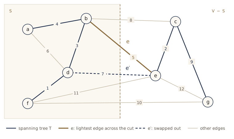
The figure starts from a spanning tree that is not minimum, which shows the exchange at work: the swap strictly improves it. Here is the same exchange in code. tree_path finds the unique path between two vertices of a tree (Lemma 4) by searching from one end and following the recorded edges back.
def tree_path(tree_edges, s, t):
    """The unique path from s to t in a tree, as a list of edges."""
    graph = adjacency(vertices_of(tree_edges), tree_edges)
    via = {s: None}                 # via[v] = the tree edge used to reach v
    stack = [s]
    while stack:
        u = stack.pop()
        for v, w in graph[u]:
            if v not in via:
                via[v] = (u, v, w)
                stack.append(v)
    path = []
    while t != s:
        u, v, w = via[t]
        path.append((u, v, w))
        t = u
    return path[::-1]

def crosses(edge, S):
    u, v, _ = edge
    return (u in S) != (v in S)

S = {"a", "b", "d", "f"}
T = [("a","b",4), ("b","d",3), ("d","f",1), ("d","e",7), ("c","e",2), ("c","g",9)]

e = min((x for x in campus if crosses(x, S)), key=lambda x: x[2])
cycle = tree_path(T, e[0], e[1]) + [e]
e_prime = next(x for x in cycle if x != e and crosses(x, S))
T_new = [x for x in T if x != e_prime] + [e]

print("lightest crossing edge e:", e)
print("cycle closed by e:       ", cycle)
print("other crossing edge e':  ", e_prime)
print("weight(T) =", weight(T), "  weight(T') =", weight(T_new),
      "  T' spanning tree:", is_spanning_tree(V, T_new))
lightest crossing edge e: ('b', 'e', 5)
cycle closed by e:        [('b', 'd', 3), ('d', 'e', 7), ('b', 'e', 5)]
other crossing edge e':   ('d', 'e', 7)
weight(T) = 26   weight(T') = 24   T' spanning tree: True
Watch out. The cut property says the lightest crossing edge is safe only for a cut that no chosen edge crosses. If \(X\) already crosses the cut, the lightest crossing edge may close a cycle with \(X\) and be useless. Also note “a lightest edge”: when several crossing edges tie, any one of them is safe, which is why a graph with repeated weights can have several different minimum spanning trees.
Kruskal’s algorithm
Kruskal’s algorithm starts with no edges and considers the edges in order of increasing weight. Each edge is added unless it would close a cycle with the edges already chosen. On the campus graph, the order is d–f (1), c–e (2), b–d (3), a–b (4), b–e (5), a–d (6), and so on. The first five are all accepted; a–d is rejected because a and d are already connected through b.
Why is this correct? We show by induction that the chosen edges \(X\) are always part of some MST. At the start \(X\) is empty, which is part of every MST. Suppose Kruskal’s algorithm now accepts \(e = \{u, v\}\). The edges in \(X\) split the vertices into connected components, and \(u\) and \(v\) lie in different ones, since \(e\) closes no cycle. Let \(S\) be the component that contains \(u\).
- No edge of \(X\) crosses \((S, V - S)\), because \(S\) is a whole component of \(X\).
- The edge \(e\) is a lightest edge crossing this cut. Any lighter crossing edge was considered earlier. At that time its endpoints were in different components too (components only grow by merging, so vertices that are apart now were apart then), so it would have been accepted and would be in \(X\), and then it would not cross.
By the cut property, \(X \cup \{e\}\) is part of some MST. At the end, \(X\) connects all the vertices: if two components of \(X\) remained, the graph, being connected, would have an edge between them, and Kruskal’s algorithm would have accepted it. So \(X\) is a spanning tree contained in an MST, which means it is an MST.
To implement this we need to know, for each candidate edge, whether its endpoints are already in the same component, and after accepting it, to merge their components. The state of the algorithm is a collection of disjoint sets — the vertex sets of the components — with three operations:
makeset(x): create a set containing only \(x\);find(x): return a name for the set containing \(x\), the same name for every member;union(x, y): merge the sets containing \(x\) and \(y\).
Kruskal’s algorithm on a graph with vertex set \(V\) and edge set \(E\) uses \(\lvert V \rvert\) makesets, \(2\lvert E \rvert\) finds (two per edge), and \(\lvert V \rvert - 1\) unions (one per accepted edge). The next section builds a structure that makes all of these fast.
A data structure for disjoint sets
Store each set as a rooted tree. Every element has a parent pointer; following parent pointers from any element leads to the root, whose parent pointer points to itself. The root is the set’s name. So find(x) climbs from \(x\) to the root, and its cost is the number of pointers followed, at most the height of the tree. union(x, y) finds the two roots and makes one point to the other.
Which root should point to which? To keep trees short, hang the shorter tree under the taller one: then the height grows only when the two trees are equally tall. Instead of maintaining heights, each element keeps a number called its rank, which starts at 0. When two roots are linked, the root of lower rank points to the root of higher rank; if the ranks are equal, either one goes under the other and the new root’s rank increases by one. This rule is union by rank. For now, the rank of a root is exactly the height of its tree.
Below is the structure in Python, with the second improvement of this section, path compression, already built in behind a switch (we explain it after Kruskal’s algorithm). The counter steps records the parent pointers that find follows, so that we can measure the work exactly.
class UnionFind:
    """Disjoint sets as parent-pointer trees: union by rank, path compression."""

    def __init__(self, elements, compress=True):
        self.parent = {x: x for x in elements}   # makeset(x) for every element
        self.rank = {x: 0 for x in elements}
        self.compress = compress
        self.steps = 0                           # parent pointers followed by find

    def find(self, x):
        root = x
        while self.parent[root] != root:         # climb to the root
            root = self.parent[root]
            self.steps += 1
        if self.compress:                        # second pass: repoint the path
            while self.parent[x] != root:
                nxt = self.parent[x]
                self.parent[x] = root
                x = nxt
        return root

    def union(self, x, y):
        """Merge the sets of x and y; return False if they were already the same set."""
        rx, ry = self.find(x), self.find(y)
        if rx == ry:
            return False
        if self.rank[rx] > self.rank[ry]:
            rx, ry = ry, rx                      # now rank[rx] <= rank[ry]
        self.parent[rx] = ry                     # lower rank goes under higher rank
        if self.rank[rx] == self.rank[ry]:
            self.rank[ry] += 1
        return True

uf = UnionFind("abcdefgh")
for x, y in [("a", "b"), ("c", "d"), ("a", "c"), ("e", "f"), ("g", "e"), ("e", "a")]:
    uf.union(x, y)
print("parent:", uf.parent)
print("rank:  ", uf.rank)
print("find(a) =", uf.find("a"), "  find(h) =", uf.find("h"))
parent: {'a': 'd', 'b': 'd', 'c': 'd', 'd': 'd', 'e': 'f', 'f': 'd', 'g': 'f', 'h': 'h'}
rank:   {'a': 0, 'b': 1, 'c': 0, 'd': 2, 'e': 0, 'f': 1, 'g': 0, 'h': 0}
find(a) = d   find(h) = h
Trace it: union(a, b) puts a under b (rank 1), union(c, d) puts c under d (rank 1), union(a, c) links the rank-1 roots b and d, making d a root of rank 2. Then e, f, g form a tree of rank 1 under f, and union(e, a) hangs that rank-1 tree under the rank-2 root d, without increasing the rank. Seven elements now form one set named d, and h is alone. Notice that a now points straight at d rather than at b: the find inside the last union compressed a’s path, as explained below.
Three properties of ranks make the analysis work. They hold for any sequence of makeset, union, and find operations.
Lemma (rank properties). (1) If \(x\) is not a root, then \(\text{rank}(x) < \text{rank}(\text{parent}(x))\). (2) A root of rank \(k\) has at least \(2^k\) elements in its tree. (3) Among \(n\) elements, at most \(n / 2^k\) have rank \(k\).
(1) When \(x\) is linked under \(y\), \(\text{rank}(x) \le \text{rank}(y)\), and if they were equal, \(y\)’s rank goes up by one. After that, \(x\) is never a root again, so its rank never changes, while \(y\)’s rank can only grow.
(2) By induction on \(k\). A rank-0 tree has at least \(1 = 2^0\) element. A root reaches rank \(k\) only when two roots of rank \(k - 1\) are linked, and by induction each brings at least \(2^{k-1}\) elements, for \(2^k\) in all. Trees never lose elements.
(3) Consider the moment a node \(x\) reaches rank \(k\). It is a root then, and by (2) it has at least \(2^k\) elements below it; call them the elements charged to \(x\). Two different nodes of rank \(k\) cannot be charged the same element \(z\): both would be ancestors of \(z\) (a node that stops being a root keeps its descendants), and by (1) ranks strictly increase on the way up from \(z\), so \(z\) has at most one ancestor of rank \(k\). So the rank-\(k\) nodes are charged disjoint groups of at least \(2^k\) elements each, and there are at most \(n / 2^k\) of them.
By (3), no rank exceeds \(\log_2 n\), since a rank \(k\) with \(2^k > n\) would need fewer than one node. By (1), a path from any element to its root passes through strictly increasing ranks, so it has at most \(\log_2 n\) edges. Therefore find and union each take \(O(\log n)\) time.
The bound is tight without path compression. The next cell builds trees of the worst shape by always merging two equal trees, then does 1,000 finds on random elements.
import random

def paired_unions(n, compress):
    """Union-by-rank structure on 0..n-1 (n a power of 2), merging equal-size sets."""
    uf = UnionFind(range(n), compress=compress)
    size = 1
    while size < n:
        for i in range(0, n, 2 * size):
            uf.union(i, i + size)
        size *= 2
    return uf

random.seed(5)
queries = [random.randrange(1024) for _ in range(1000)]
for compress in [False, True]:
    uf = paired_unions(1024, compress)
    uf.steps = 0
    for x in queries:
        uf.find(x)
    print(f"compress={compress!s:5}  max rank {max(uf.rank.values())}   "
          f"pointers followed by 1,000 finds: {uf.steps:,}")
compress=False  max rank 10   pointers followed by 1,000 finds: 4,994
compress=True   max rank 10   pointers followed by 1,000 finds: 1,695
With 1,024 elements the maximum rank is exactly \(\log_2 1024 = 10\), and without compression a find on a random element follows about 5 pointers, half the height. With compression the same 1,000 finds follow 1,695 pointers, fewer than two per find: early finds flatten the paths they touch, and later finds reach the root almost at once.
Kruskal’s algorithm in code
With union–find in hand, Kruskal’s algorithm is a sort and a loop.
def kruskal(vertices, edges, trace=False):
    """Minimum spanning tree, as a list of edges, of a connected graph (edge list)."""
    uf = UnionFind(vertices)
    tree = []
    for u, v, w in sorted(edges, key=lambda e: e[2]):   # increasing weight
        if uf.find(u) != uf.find(v):                     # different components
            tree.append((u, v, w))
            uf.union(u, v)
            if trace: print(f"  add  {u}-{v} ({w})")
        elif trace:
            print(f"  skip {u}-{v} ({w})")
        if len(tree) == len(vertices) - 1:
            break                                        # a spanning tree is complete
    return tree

mst = kruskal(V, campus, trace=True)
print("MST weight:", weight(mst))
  add  d-f (1)
  add  c-e (2)
  add  b-d (3)
  add  a-b (4)
  add  b-e (5)
  skip a-d (6)
  skip d-e (7)
  skip b-c (8)
  add  c-g (9)
MST weight: 24
The tree has weight 24, the same edges as six_good above. Three edges were skipped because both endpoints were already in the same component; the last three edges were never looked at, since the tree was complete after c–g. (The early exit does not change the answer; it only saves time.)
Running time. Sorting the edges takes \(O(\lvert E \rvert \log \lvert E \rvert)\) time, which is \(O(\lvert E \rvert \log \lvert V \rvert)\) because \(\lvert E \rvert \le \lvert V \rvert^2\) and so \(\log \lvert E \rvert \le 2 \log \lvert V \rvert\). The loop does \(2\lvert E \rvert\) finds and \(\lvert V \rvert - 1\) unions at \(O(\log \lvert V \rvert)\) each. In total, Kruskal’s algorithm runs in \(O(\lvert E \rvert \log \lvert V \rvert)\) time.
Path compression
If the sort dominates, why improve union–find further? Because sometimes there is no sort to pay for: the edges may arrive already sorted, or the weights may be small integers that can be sorted in linear time. Then the finds are the bottleneck. Union–find is also used on its own in many other algorithms, where it is the whole cost.
Path compression is a small change to find: after climbing from \(x\) to the root, go over the path a second time and make every node on it point directly at the root. That is the second loop in our find. It at most doubles the cost of that find, and it makes later finds on any of those nodes, or on anything below them, much shorter.
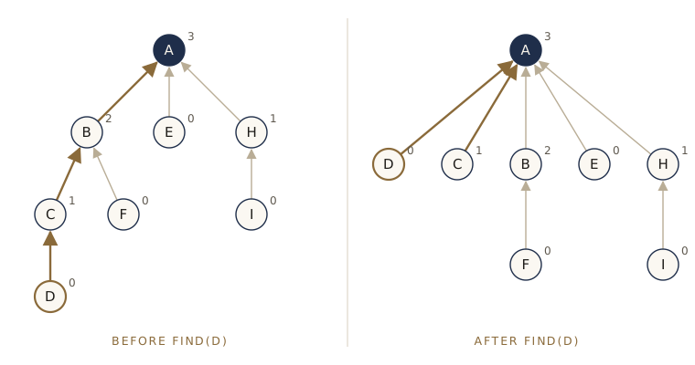
find(D). The three pointers on the path D → C → B → A are followed once; afterward D and C point straight at the root. Ranks (the small numbers) do not change, even though they no longer equal heights.Path compression changes parent pointers only inside trees; it never changes which elements are roots or what their ranks are, because union looks only at roots and their ranks. So the sequence of roots and ranks is exactly what it would have been without compression, and the three rank properties still hold. (Property (1) survives because the new parent is an ancestor, and ranks increase going up.) What changes is the analysis: a single find can still take \(\log n\) steps, but a long find leaves a flat tree behind, so expensive finds cannot keep happening. We need to bound the total cost of a sequence of operations, not each one.
Definition. The amortized cost of an operation is the total cost of a sequence of operations divided by the number of operations, in the worst case over all sequences.
The bound involves a function that grows so slowly it is at most 5 for any input you could store. The iterated logarithm \(\log^* n\) is the number of times you must apply \(\log_2\) to \(n\) before the result is at most 1.
import math

def log_star(n):
    """Number of times log2 must be applied to n to bring it down to 1 or less."""
    count = 0
    while n > 1:
        n = math.log2(n)
        count += 1
    return count

for n in [2, 16, 65536, 2 ** 65536]:
    label = "2^65536" if n == 2 ** 65536 else f"{n:,}"
    print(f"log* {label:>8} = {log_star(n)}")
log*        2 = 1
log*       16 = 3
log*   65,536 = 4
log*  2^65536 = 5
Theorem. With union by rank and path compression, any sequence of \(m\) find operations on \(n\) elements takes \(O((m + n) \log^* n)\) time in total.
Here is a sketch of the argument, which uses a bank-account style of accounting.
Rank groups. Split the possible nonzero ranks into groups of the form \(\{k + 1, k + 2, \dots, 2^k\}\), starting from \(k = 0\) and letting each group’s top \(2^k\) be the next group’s \(k\): the groups are \(\{1\}\), \(\{2\}\), \(\{3, 4\}\), \(\{5, \dots, 16\}\), \(\{17, \dots, 65536\}\), and so on. Ranks never exceed \(\log_2 n\), so only about \(\log^* n\) groups are ever used.
Allowances. When a node stops being a root, its rank is frozen forever. At that moment, give it an allowance of \(2^k\) dollars if its rank lies in the group \(\{k+1, \dots, 2^k\}\). By rank property (3), the number of nodes with rank above \(k\) is at most
\[\frac{n}{2^{k+1}} + \frac{n}{2^{k+2}} + \cdots \le \frac{n}{2^k},\]so the nodes in one group receive at most \(n\) dollars in all, and the total paid out over all groups is at most \(n \log^* n\).
Paying for a find. A find costs one unit per pointer followed. Go up the path and look at each node \(x\) on it. If \(x\) is the root or a child of the root, or if its parent’s rank is in a higher group than its own rank, the find itself pays for \(x\); there are at most \(\log^* n + 2\) such nodes on any path, since ranks increase along the path and can change group only \(\log^* n\) times. Otherwise \(x\) pays one dollar from its allowance.
The allowance suffices. Each time \(x\) pays, it was not a child of the root, so compression gives it a new parent, the root, whose rank is larger than its old parent’s rank. So each payment raises the rank of \(x\)’s parent by at least one. If \(x\)’s rank is in the group \(\{k+1, \dots, 2^k\}\), then after at most \(2^k\) payments its parent’s rank has left that group, and from then on the find pays for \(x\). The allowance of \(2^k\) dollars covers it.
Adding up: \(m\) finds cost at most \(m(\log^* n + 2)\) paid by the finds, plus at most \(n \log^* n\) paid from allowances, which is \(O((m + n)\log^* n)\). Unions cost two finds plus a constant, so they are covered too.
Note. The true amortized cost is even smaller. Tarjan showed that union by rank with path compression costs \(O(\alpha(n))\) per operation, where \(\alpha\) is the inverse of Ackermann’s function, which grows far more slowly than \(\log^* n\), and that for this kind of structure the bound cannot be improved. For all practical purposes, each operation takes constant time.
Prim’s algorithm
The cut property allows more than one algorithm. Any procedure of this form produces an MST:
- Start with no edges, \(X = \emptyset\).
- While \(X\) has fewer than \(\lvert V \rvert - 1\) edges: choose any cut \((S, V - S)\) that no edge of \(X\) crosses, and add to \(X\) a lightest edge crossing it.
Kruskal’s algorithm is one instance, with \(S\) the component of one endpoint of the next edge. Prim’s algorithm is another: it keeps \(X\) connected, a single tree growing from a start vertex, and always uses the cut between the tree’s vertices \(S\) and everything else. At each step it adds the lightest edge leaving the tree.
To find that edge quickly, give every vertex \(v\) outside the tree a cost, the weight of the lightest edge from the tree to \(v\):
\[\text{cost}(v) = \min_{u \in S} w(u, v).\]Each step moves the vertex of smallest cost into the tree, then lowers the costs of its neighbors where the new vertex offers a lighter edge. This is Dijkstra’s algorithm almost line for line. The only difference is the key in the priority queue: Dijkstra’s key for \(v\) is the length of a whole path from the start, \(\text{dist}(u) + w(u, v)\), while Prim’s key is the weight of a single edge, \(w(u, v)\).
Python’s heapq has no decrease-key operation. The usual workaround is to push a new entry whenever a cost goes down and to skip entries for vertices that are already in the tree when they are popped.
import heapq

def prim(graph, start, trace=False):
    """MST of a connected graph {u: [(v, w), ...]}, grown from start: (prev, cost)."""
    cost = {u: math.inf for u in graph}
    prev = {u: None for u in graph}
    cost[start] = 0
    in_tree = set()
    heap = [(0, start)]
    while heap:
        c, v = heapq.heappop(heap)
        if v in in_tree:
            continue                      # stale entry: v is already in the tree
        in_tree.add(v)
        if trace:
            print(f"  add {v} via {prev[v]}-{v} ({c})" if prev[v] else f"  start: {v}")
        for z, w in graph[v]:
            if z not in in_tree and w < cost[z]:
                cost[z] = w               # a lighter edge from the tree to z
                prev[z] = v
                heapq.heappush(heap, (w, z))
    return prev, cost

def prim_edges(prev, cost):
    """The tree edges (prev[v], v, cost[v]) recorded by prim."""
    return [(prev[v], v, cost[v]) for v in prev if prev[v] is not None]

prev, cost = prim(G, "a", trace=True)
print("MST weight:", weight(prim_edges(prev, cost)))
  start: a
  add b via a-b (4)
  add d via b-d (3)
  add f via d-f (1)
  add e via b-e (5)
  add c via e-c (2)
  add g via c-g (9)
MST weight: 24
Prim’s algorithm finds the same tree as Kruskal’s, weight 24, but in a different order: it grows outward from a, so it must take a–b (4) before it can reach the cheap edge d–f (1). The prev pointers describe the whole tree, just as Dijkstra’s prev pointers describe the shortest-path tree.
Watch out. The test
z not in in_treematters. Once a vertex is in the tree, its edge to the tree is final. Without the test, a vertex added later could offer an even lighter edge to a vertex already in the tree and overwrite itspreventry, and theprevpointers would no longer describe the tree that was actually built.
Correctness. Each step adds a lightest edge across the cut \((S, V - S)\), where \(S\) is the set of tree vertices. No chosen edge crosses this cut, because all chosen edges have both endpoints in \(S\). So the cut property applies at every step.
Running time. The same as Dijkstra’s algorithm with the same priority queue. With a binary heap and lazy deletion, each edge causes at most two pushes (one from each end), so the heap holds \(O(\lvert E \rvert)\) entries and every heap operation costs \(O(\log \lvert E \rvert) = O(\log \lvert V \rvert)\). The total is \(O((\lvert V \rvert + \lvert E \rvert) \log \lvert V \rvert)\), the same as Kruskal’s algorithm on a connected graph. On a dense graph, where \(\lvert E \rvert\) is close to \(\lvert V \rvert^2\), an unsorted array in place of the heap gives \(O(\lvert V \rvert^2)\), which is better.
Testing against brute force
Our two algorithms agree on one graph. To gain more confidence, compare both with a brute-force search on many small random graphs. The brute force tries every set of \(n - 1\) edges, keeps those that form a spanning tree, and returns the lightest. The random graphs use small integer weights, so ties are common and a graph may have several MSTs; we compare weights, not edge sets.
from itertools import combinations

def brute_force_mst_weight(vertices, edges):
    """Weight of a lightest spanning tree, by trying every set of n - 1 edges."""
    return min(weight(subset) for subset in combinations(edges, len(vertices) - 1)
               if is_spanning_tree(vertices, list(subset)))

def random_connected_graph(n, extra, max_w):
    """Random connected graph on 0..n-1: a random spanning tree plus `extra` edges."""
    pairs = set()
    for v in range(1, n):
        pairs.add((random.randrange(v), v))          # guarantees connectivity
    all_pairs = [(u, v) for u in range(n) for v in range(u + 1, n)]
    others = [p for p in all_pairs if p not in pairs]
    pairs.update(random.sample(others, min(extra, len(others))))
    return [(u, v, random.randint(1, max_w)) for u, v in sorted(pairs)]

random.seed(431)
trials = 300
for _ in range(trials):
    n = random.randint(2, 7)
    edges = random_connected_graph(n, random.randint(0, 6), max_w=6)
    verts = list(range(n))
    k = kruskal(verts, edges)
    p = prim_edges(*prim(adjacency(verts, edges), 0))
    assert is_spanning_tree(verts, k) and is_spanning_tree(verts, p)
    assert weight(k) == weight(p) == brute_force_mst_weight(verts, edges)
print(f"Kruskal, Prim, and brute force agree on {trials} random graphs")
Kruskal, Prim, and brute force agree on 300 random graphs
A randomized algorithm for minimum cut
Spanning trees and cuts are closely connected, and here is a surprising use of that connection. In an unweighted graph, a minimum cut is a cut crossed by as few edges as possible; its size measures how robustly the graph is connected.
Run Kruskal’s algorithm with the edges in a uniformly random order, and stop just before the last edge would be added. At that point there are exactly two components, and they define a cut. The claim is that this cut is a minimum cut with probability at least \(2/(n(n-1))\), where \(n\) is the number of vertices.
Sketch. Let \(C\) be the size of a minimum cut, and fix one minimum cut. When the chosen edges form \(k\) components, every component has at least \(C\) edges leaving it (otherwise the cut around that component would be smaller than the minimum). So at least \(kC/2\) edges join different components (each such edge leaves two components), and the next edge Kruskal adds is equally likely to be any of them. At most \(C\) of them cross our fixed minimum cut, so the chance of adding one is at most \(C/(kC/2) = 2/k\). The algorithm avoids the cut through every step, from \(k = n\) down to \(k = 3\), with probability at least
\[\frac{n-2}{n} \cdot \frac{n-3}{n-1} \cdot \frac{n-4}{n-2} \cdots \frac{2}{4} \cdot \frac{1}{3} = \frac{2}{n(n-1)},\]since almost every factor cancels. If it never adds an edge of the cut, the two final components are exactly the two sides of the cut.
A success probability of about \(2/n^2\) sounds small, but repetition fixes that: after \(n^2\) independent runs, the chance that all of them miss is at most \((1 - 2/n^2)^{n^2} \le e^{-2}\), and \(n^2 \ln n\) runs push it down to at most \(1/n^2\). Keep the smallest cut found. This algorithm is known as Karger’s contraction algorithm, and refinements of it are among the fastest ways known to compute minimum cuts. Here it is on a graph made of two groups of four vertices, each group fully connected, joined by two edges, so the minimum cut has size 2.
def random_kruskal_cut(vertices, edges):
    """Kruskal on a random edge order, stopped at two components: the cut size."""
    order = edges[:]
    random.shuffle(order)
    uf = UnionFind(vertices)
    components = len(vertices)
    for u, v, _ in order:
        if components == 2:
            break
        if uf.union(u, v):
            components -= 1
    side = {x for x in vertices if uf.find(x) == uf.find(vertices[0])}
    return sum(1 for u, v, _ in edges if (u in side) != (v in side))

clusters = [(u, v, 1) for group in [range(4), range(4, 8)]
            for u, v in combinations(group, 2)] + [(0, 4, 1), (1, 5, 1)]
random.seed(2)
runs = [random_kruskal_cut(list(range(8)), clusters) for _ in range(2000)]
print("cut sizes seen:", sorted(set(runs)))
print(f"fraction of runs that found the minimum cut: {runs.count(2) / len(runs):.2f}"
      f"   (guarantee: {2 / (8 * 7):.3f})")
cut sizes seen: [2, 3, 4, 5, 6, 7, 8]
fraction of runs that found the minimum cut: 0.21   (guarantee: 0.036)
About one run in five finds the minimum cut of size 2, roughly six times the guaranteed 0.036; the other runs return larger cuts, up to 8. The guarantee is a worst-case lower bound that holds for every graph, and a particular graph usually does better. Keeping the smallest cut over a few dozen runs finds the minimum here with near certainty.
Huffman encoding
Variable-length codes
Suppose you must store a long string over a small alphabet in binary. The simplest scheme gives every symbol a codeword of the same length: with 7 distinct symbols, 3 bits each. But if some symbols are much more common than others, it pays to give the common ones short codewords and the rare ones long codewords.
Our running example is the 26-character string tennessee sees seven trees, in which “e” appears 10 times and “r” once. A fixed-length code needs \(26 \times 3 = 78\) bits.
Variable-length codes bring a danger: the encoded bits might be ambiguous. If a is 0, b is 01, and c is 10, then 010 could be “a c” or “b a”. The fix is to require that no codeword be a prefix of another. Such a code is called a prefix-free code. Reading a prefix-free code from left to right, the moment the bits read so far match a codeword, that codeword is the only one that can match, so decoding is unambiguous.
A prefix-free code is a binary tree. Put the symbols at the leaves, and read the codeword of a symbol off the path from the root: 0 for each step to a left child, 1 for each step to a right child. Because symbols sit only at leaves, no codeword is the prefix of another. To decode, start at the root, follow one edge per bit, and whenever you reach a leaf, output its symbol and jump back to the root. In an optimal code, every internal node has exactly two children: an internal node with a single child could be removed, which shortens every codeword beneath it. A tree in which every node has zero or two children is a full binary tree.
The cost of a tree
Let the symbols have frequencies \(f_1, \dots, f_n\) (counts, or probabilities). A symbol at depth \(d_i\) has a codeword of \(d_i\) bits, so the encoded length is
\[\text{cost}(T) = \sum_{i=1}^{n} f_i \cdot d_i .\]There is a second way to count the same bits, which is the key to the algorithm. Give every internal node a frequency too: the sum of the frequencies of the leaves below it. Encoding a symbol walks from the root down to its leaf and writes one bit per node entered. A node with frequency \(f\) is entered once for each of the \(f\) occurrences of the symbols below it. So
\[\text{cost}(T) = \text{the sum of the frequencies of all nodes except the root.}\]The greedy merge
The two least frequent symbols should sit at the very bottom of the tree, as siblings (we prove this below). Huffman’s algorithm makes that choice first and repeats: take the two trees of smallest frequency, make them the two children of a new node whose frequency is their sum, and put the new tree back. Start with one single-leaf tree per symbol and stop when one tree remains. A priority queue does the bookkeeping.
from collections import Counter

def huffman_tree(freq):
    """Huffman tree for {symbol: frequency}, plus the list of merged frequencies.
    A leaf is a symbol; an internal node is a pair (left, right)."""
    heap = [(f, i, sym) for i, (sym, f) in enumerate(sorted(freq.items()))]
    heapq.heapify(heap)
    next_id = len(heap)                  # tie-breaker: heapq never compares two trees
    merged = []
    while len(heap) > 1:
        f1, _, t1 = heapq.heappop(heap)  # the two least frequent trees
        f2, _, t2 = heapq.heappop(heap)
        heapq.heappush(heap, (f1 + f2, next_id, (t1, t2)))
        next_id += 1
        merged.append(f1 + f2)
    return heap[0][2], merged

def codewords(tree, prefix=""):
    """{symbol: codeword} for a code tree: left edges are 0, right edges are 1."""
    if not isinstance(tree, tuple):
        return {tree: prefix or "0"}     # a one-symbol alphabet still needs one bit
    codes = codewords(tree[0], prefix + "0")
    codes.update(codewords(tree[1], prefix + "1"))
    return codes

text = "tennessee sees seven trees"
freq = Counter(text)
tree, merged = huffman_tree(freq)
codes = codewords(tree)
for sym in sorted(codes, key=lambda s: (-freq[s], s)):
    name = "space" if sym == " " else sym
    print(f"{name:>6}  count {freq[sym]:2d}  codeword {codes[sym]}")
print("merged frequencies:", merged)
     e  count 10  codeword 11
     s  count  6  codeword 01
 space  count  3  codeword 100
     n  count  3  codeword 101
     t  count  2  codeword 000
     r  count  1  codeword 0010
     v  count  1  codeword 0011
merged frequencies: [2, 4, 6, 10, 16, 26]
Read the merges off the list: r and v (1 + 1 = 2), then t with that pair (2 + 2 = 4), then space and n (3 + 3 = 6), then the 4-tree with s (4 + 6 = 10), then e with the 6-tree (10 + 6 = 16), and finally the two remaining trees (10 + 16 = 26). “e” gets two bits, the rare letters four.
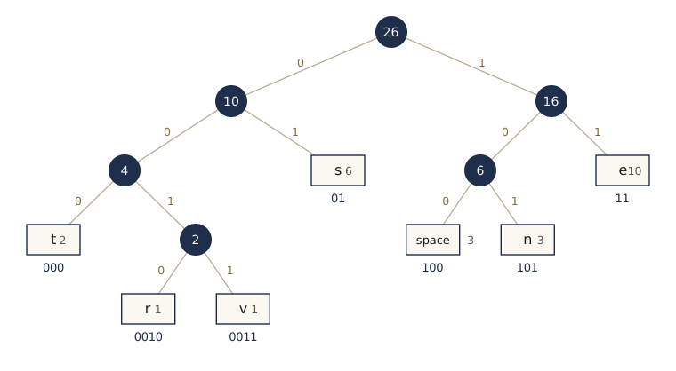
tennessee sees seven trees. Each internal node carries the sum of the frequencies below it; adding up all the numbers except the root's 26 gives the encoded length, 64 bits.Now check the claims: the code is prefix-free, the two cost formulas agree, and decoding recovers the text.
def is_prefix_free(codes):
    """No codeword is a prefix of another.
    After sorting, a prefix would sit right before a word that starts with it."""
    words = sorted(codes.values())
    return all(not b.startswith(a) for a, b in zip(words, words[1:]))

def encode(text, codes):
    return "".join(codes[ch] for ch in text)

def decode(bits, tree):
    out, node = [], tree
    for b in bits:
        node = node[int(b)]                  # 0 = left child, 1 = right child
        if not isinstance(node, tuple):      # reached a leaf
            out.append(node)
            node = tree
    return "".join(out)

bits = encode(text, codes)
print("prefix-free:", is_prefix_free(codes))
print("sum of f_i * depth_i:", sum(freq[s] * len(codes[s]) for s in freq))
print("sum of merged frequencies:", sum(merged))
print("encoded length:", len(bits), "bits; a fixed 3-bit code needs", 3 * len(text))
print("round trip ok:", decode(bits, tree) == text)
prefix-free: True
sum of f_i * depth_i: 64
sum of merged frequencies: 64
encoded length: 64 bits; a fixed 3-bit code needs 78
round trip ok: True
The Huffman code uses 64 bits, 18% fewer than the fixed-length code, and both ways of computing the cost give 64. The sum of the merged values is a third way to get the same number. Each merged value is the frequency of one internal node, root included, and that frequency is the sum of its two children’s frequencies; adding over all internal nodes therefore counts every node except the root exactly once, which is the second cost formula.
Running time. With \(n\) symbols the algorithm does \(n - 1\) merges, each costing a constant number of heap operations, so it takes \(O(n \log n)\) time with a binary heap, plus the time to count frequencies in the input.
Why merging the two rarest symbols is optimal
Lemma. Let \(f_1\) and \(f_2\) be the two smallest frequencies. Some optimal tree has the symbols 1 and 2 as sibling leaves at maximum depth.
The idea is an exchange: moving a rarer symbol deeper never costs more. Take any optimal tree. It is full, so its deepest internal node has two children, and both are leaves at maximum depth; call their symbols \(x\) and \(y\). Swap symbol 1 with \(x\). If symbol 1 was at depth \(d_1\) and \(x\) at depth \(d_x \ge d_1\), the cost changes by
\[f_1 d_x + f_x d_1 - f_1 d_1 - f_x d_x = -(f_x - f_1)(d_x - d_1) \le 0,\]because \(f_x \ge f_1\) and \(d_x \ge d_1\). So the tree stays optimal. Swapping symbol 2 with \(y\) in the same way puts 1 and 2 together as siblings at maximum depth.
Theorem. Huffman’s algorithm produces an optimal prefix-free code.
The proof is by induction on the number of symbols \(n\); for \(n = 2\) the only full tree is a root with two leaves. For larger \(n\), by the lemma we may restrict attention to trees in which symbols 1 and 2 are siblings. Given such a tree \(T\), delete the two sibling leaves, so that their parent becomes a leaf for a new symbol of frequency \(f_1 + f_2\); call the result \(T'\). By the second cost formula, \(T\) counts every node of \(T'\) except its root, plus the two deleted leaves:
\[\text{cost}(T) = \text{cost}(T') + f_1 + f_2 .\]The term \(f_1 + f_2\) does not depend on the shape of the tree, so \(T\) is optimal among such trees exactly when \(T'\) is optimal for the \(n - 1\) frequencies \(f_1 + f_2, f_3, \dots, f_n\). Huffman’s algorithm merges 1 and 2 and then runs on precisely that smaller problem, where it is optimal by induction.
A brute-force check: every full binary tree can be built by some sequence of merges, and a sequence of merges costs the sum of the merged frequencies. So trying all sequences of merges finds the true optimum. That is exponential, but fine for up to seven symbols.
from functools import cache

@cache
def best_merge_cost(freqs):
    """Cheapest total over all sequences of merges (freqs is a sorted tuple)."""
    if len(freqs) == 1:
        return 0
    best = math.inf
    for i, j in combinations(range(len(freqs)), 2):
        rest = [f for k, f in enumerate(freqs) if k != i and k != j]
        merged_one = freqs[i] + freqs[j]
        smaller = tuple(sorted(rest + [merged_one]))
        best = min(best, merged_one + best_merge_cost(smaller))
    return best

random.seed(7)
for _ in range(500):
    fs = [random.randint(1, 30) for _ in range(random.randint(2, 7))]
    _, merged = huffman_tree(dict(enumerate(fs)))
    assert sum(merged) == best_merge_cost(tuple(sorted(fs)))
print("Huffman cost equals the brute-force optimum on 500 random frequency lists")
Huffman cost equals the brute-force optimum on 500 random frequency lists
Entropy
How far can compression go? Information theory gives an answer in terms of the probabilities of the symbols. If symbol \(i\) occurs with probability \(p_i\), the entropy of the distribution is
\[H = \sum_{i=1}^{n} p_i \log_2 \frac{1}{p_i} .\]It measures unpredictability in bits per symbol. A fair coin has entropy \(\tfrac12 \log_2 2 + \tfrac12 \log_2 2 = 1\) bit. A coin that lands heads three times out of four has entropy \(\tfrac34 \log_2 \tfrac43 + \tfrac14 \log_2 4 \approx 0.811\): it is more predictable, so each flip carries less information. A coin that always lands heads has entropy 0.
A standard result of information theory, which we do not prove here, says that the average codeword length \(L\) of any prefix-free code is at least \(H\), and that the Huffman code achieves \(H \le L < H + 1\). When every \(p_i\) is a power of \(1/2\), Huffman gives symbol \(i\) a codeword of exactly \(\log_2(1/p_i)\) bits and \(L = H\).
def entropy(probs):
    return sum(p * math.log2(1 / p) for p in probs if p > 0)

probs = [freq[s] / len(text) for s in freq]
print(f"fair coin: {entropy([0.5, 0.5]):.3f}   3/4 coin: {entropy([0.75, 0.25]):.3f}")
print(f"our text: entropy {entropy(probs):.3f} bits/symbol, "
      f"Huffman {len(bits) / len(text):.3f} bits/symbol")
fair coin: 1.000   3/4 coin: 0.811
our text: entropy 2.384 bits/symbol, Huffman 2.462 bits/symbol
For our text the Huffman code spends about 0.08 bits per symbol more than the entropy, well inside the guarantee of less than one.
Note. Huffman’s algorithm is optimal among codes that assign one codeword to each symbol, independently of its neighbors. Real compressors do better on real data by exploiting context — in English, “q” is nearly always followed by “u” — and by coding longer blocks at a time, but Huffman coding still appears as a final stage in widely used formats.
Horn formulas
Implications and negative clauses
Logical reasoning in programs often has a simple shape: a list of facts, a list of rules of the form “if these hold, then that holds”, and a list of constraints that certain things cannot all hold together. Horn formulas capture exactly this shape, and they can be solved greedily.
A Boolean variable takes the value true or false. A literal is a variable \(x\) or its negation \(\bar{x}\) (“not \(x\)”). A Horn formula is a collection of clauses of two kinds:
- Implications: an AND of zero or more variables on the left and one variable on the right, such as \((w \wedge y) \Rightarrow z\), “if \(w\) and \(y\) are true, then \(z\) is true”. With nothing on the left, \(\Rightarrow x\) says simply that \(x\) is true: a fact.
- Pure negative clauses: an OR of one or more negated variables, such as \((\bar{u} \vee \bar{v})\), “\(u\) and \(v\) are not both true”.
An assignment of true or false to every variable is a satisfying assignment if it makes every clause true. The problem: given a Horn formula, find a satisfying assignment or report that none exists.
Here is a small formula about a road in winter. The facts say it is raining and cold; the rules say what follows; the negative clauses say the road is not closed, and that it is not both icy and dark.
\[\Rightarrow \text{rain}, \quad \Rightarrow \text{cold}, \quad \text{rain} \Rightarrow \text{wet}, \quad (\text{wet} \wedge \text{cold}) \Rightarrow \text{icy}, \quad \text{icy} \Rightarrow \text{salted}, \quad (\text{icy} \wedge \text{dark}) \Rightarrow \text{closed},\] \[(\overline{\text{closed}}), \quad (\overline{\text{icy}} \vee \overline{\text{dark}}).\]In code, an implication is a pair (premises, conclusion) and a negative clause is a tuple of the variables that appear negated. We describe an assignment by the set of variables that are true.
road_rules = [
    ((), "rain"),                 # => rain            (a fact)
    ((), "cold"),                 # => cold
    (("rain",), "wet"),           # rain => wet
    (("wet", "cold"), "icy"),     # (wet and cold) => icy
    (("icy",), "salted"),         # icy => salted
    (("icy", "dark"), "closed"),  # (icy and dark) => closed
]
road_limits = [
    ("closed",),                  # (not closed)
    ("icy", "dark"),              # (not icy or not dark)
]
The stingy algorithm
The two kinds of clauses pull in opposite directions: implications push variables toward true, negative clauses toward false. The greedy strategy is to set variables to true as reluctantly as possible. Start with every variable false. While some implication is violated (all its premises are true but its conclusion is false), set its conclusion to true. When no implication is violated, check the negative clauses; if one fails, report that the formula cannot be satisfied.
def horn_sat_simple(implications, negatives):
    """Stingy greedy algorithm: the set of true variables, or None if unsatisfiable."""
    true = set()
    changed = True
    while changed:                                   # until every implication holds
        changed = False
        for premises, conclusion in implications:
            if conclusion not in true and all(p in true for p in premises):
                true.add(conclusion)                 # forced, or the implication fails
                changed = True
    for clause in negatives:
        if all(x in true for x in clause):           # every literal "not x" is false
            return None
    return true

print(sorted(horn_sat_simple(road_rules, road_limits)))
print(horn_sat_simple(road_rules + [((), "dark")], road_limits))   # add: it is dark
['cold', 'icy', 'rain', 'salted', 'wet']
None
The facts force rain and cold; then wet, icy, and salted follow in turn. Nothing forces dark, so it stays false, closed stays false, and both negative clauses hold. Adding the fact \(\Rightarrow \text{dark}\) forces closed as well, the clause \((\overline{\text{closed}})\) fails, and the formula has no satisfying assignment.
Why it is correct
If the algorithm returns an assignment, it satisfies every implication (the loop only stops when none is violated) and every negative clause (it checked them). The real question is the other answer: when the algorithm reports failure, could some other assignment have worked? No, because of an invariant.
Lemma. Every variable that the stingy algorithm sets to true is true in every satisfying assignment.
By induction on the order in which variables are set. Suppose the algorithm sets \(z\) to true because of an implication \((x_1 \wedge \dots \wedge x_k) \Rightarrow z\) whose premises are all already true. By induction each \(x_i\) is true in every satisfying assignment, so every satisfying assignment must make \(z\) true as well, or the implication fails. (For a fact, \(k = 0\), and \(z\) is true in every satisfying assignment directly.)
Now suppose a negative clause \((\bar{x}_1 \vee \dots \vee \bar{x}_k)\) fails at the end, meaning all of \(x_1, \dots, x_k\) were set to true. By the lemma, every satisfying assignment makes them all true and so violates this clause. So there is no satisfying assignment, and the answer “unsatisfiable” is correct.
The lemma says more: when the formula is satisfiable, the algorithm returns the satisfying assignment with the fewest true variables, and every satisfying assignment includes it.
Linear time
The simple version rescans every implication after each change. Each pass costs time proportional to the length of the formula, and there can be as many passes as variables, so the worst case is quadratic. We can do better by never looking at an implication until it might have become violated.
For each implication, keep a counter of how many of its premises are still false. For each variable, keep the list of implications in which it is a premise. When a variable becomes true, walk its list and decrement those counters; when a counter reaches zero, all premises of that implication are true, so its conclusion is forced. A queue holds the variables that have been forced but not yet processed.
from collections import defaultdict, deque

def horn_sat(implications, negatives):
    """Stingy algorithm in time linear in the length of the formula."""
    waiting = [len(set(prem)) for prem, _ in implications]   # premises still false
    uses = defaultdict(list)               # variable -> implications with it as premise
    for i, (premises, _) in enumerate(implications):
        for p in set(premises):
            uses[p].append(i)
    queue = deque(c for (_, c), k in zip(implications, waiting) if k == 0)   # facts
    true = set()
    while queue:
        x = queue.popleft()
        if x in true:
            continue
        true.add(x)
        for i in uses[x]:
            waiting[i] -= 1
            if waiting[i] == 0:            # all premises true: the conclusion is forced
                queue.append(implications[i][1])
    for clause in negatives:
        if all(x in true for x in clause):
            return None
    return true

print(sorted(horn_sat(road_rules, road_limits)))
print(horn_sat(road_rules + [((), "dark")], road_limits))
['cold', 'icy', 'rain', 'salted', 'wet']
None
Running time. Building the counters and lists takes one pass over the implications. Each variable enters true at most once, and its list of uses is walked only then, so the decrements add up to the total number of premise occurrences. Each implication’s counter reaches zero at most once, so each conclusion is queued at most once from a counter, plus once for each fact. The final check reads each negative clause once. Everything is proportional to the length of the formula, plus the number of variables.
Finally, compare both versions with brute force on random small formulas. The brute force lists every satisfying assignment, so we can check the lemma too: the greedy answer must be contained in every satisfying assignment.
from itertools import product

def satisfies(true, implications, negatives):
    return (all(c in true or not all(p in true for p in prem)
                for prem, c in implications)
            and all(not all(x in true for x in cl) for cl in negatives))

def random_horn(variables, n_imp, n_neg):
    imps = [(tuple(random.sample(variables, random.randint(0, 2))),
             random.choice(variables)) for _ in range(n_imp)]
    negs = [tuple(random.sample(variables, random.randint(1, 3))) for _ in range(n_neg)]
    return imps, negs

random.seed(8)
variables = list("uvwxyz")
counts = Counter()
for _ in range(1000):
    imps, negs = random_horn(variables, random.randint(1, 8), random.randint(0, 3))
    solutions = [t for bits in product([False, True], repeat=len(variables))
                 for t in [{v for v, b in zip(variables, bits) if b}]
                 if satisfies(t, imps, negs)]
    greedy = horn_sat(imps, negs)
    assert greedy == horn_sat_simple(imps, negs)
    assert (greedy is None) == (not solutions)
    assert greedy is None or all(greedy <= s for s in solutions)   # the lemma
    counts["satisfiable" if solutions else "unsatisfiable"] += 1
print(dict(counts), "- all checks passed")
{'satisfiable': 845, 'unsatisfiable': 155} - all checks passed
Note. Horn formulas are the logical core of logic programming languages such as Prolog, and of database query languages built on rules. Satisfiability of general Boolean formulas, where a clause may contain any mix of positive and negative literals, is a different story: it is NP-complete (module 07), and no efficient algorithm for it is known. Horn formulas are a special case where a greedy rule suffices.
Set cover
The problem
Many planning problems ask for the fewest resources that together serve everyone: the fewest fire stations so that every neighborhood is within reach of one, the fewest people on a team so that every required skill is present, the fewest test cases that together exercise every line of a program. In the abstract:
Definition. In the set cover problem, the input is a set \(B\) of \(n\) elements and a list of subsets \(S_1, \dots, S_m\) of \(B\) whose union is \(B\). The goal is to choose as few of the subsets as possible so that their union is still \(B\). The chosen subsets form a cover.
There is an obvious greedy rule: repeatedly choose the set that covers the largest number of elements not yet covered.
def greedy_set_cover(universe, sets):
    """Greedy set cover; `sets` maps names to sets. Returns chosen names in order."""
    uncovered = set(universe)
    chosen = []
    while uncovered:
        best = max(sets, key=lambda name: len(sets[name] & uncovered))
        if not sets[best] & uncovered:
            raise ValueError("the sets do not cover the universe")
        chosen.append(best)
        uncovered -= sets[best]
    return chosen

def optimal_set_cover(universe, sets):
    """Smallest cover, by trying all collections of 1, 2, 3, ... sets."""
    names = list(sets)
    for k in range(1, len(names) + 1):
        for combo in combinations(names, k):
            if set().union(*(sets[c] for c in combo)) >= set(universe):
                return list(combo)
Greedy is not optimal
Here is an instance with 14 elements, arranged in two rows of seven. Two sets, R1 and R2, are the rows. Three more sets, C1, C2, and C3, are blocks of columns of widths 4, 2, and 1.
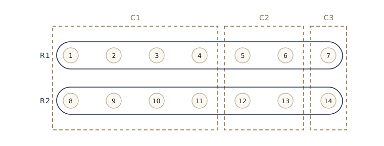
universe = range(1, 15)
blocks = {
    "R1": set(range(1, 8)),                 # top row
    "R2": set(range(8, 15)),                # bottom row
    "C1": {1, 2, 3, 4, 8, 9, 10, 11},       # columns 1-4
    "C2": {5, 6, 12, 13},                   # columns 5-6
    "C3": {7, 14},                          # column 7
}
print("greedy: ", greedy_set_cover(universe, blocks))
print("optimal:", optimal_set_cover(universe, blocks))
greedy:  ['C1', 'C2', 'C3']
optimal: ['R1', 'R2']
Greedy takes C1 because it covers 8 new elements and each row only 7. After that, each row would add only 3 new elements while C2 adds 4, and in the last round C3 adds 2 against 1 for each row. Every step was locally best, and the result uses three sets where two suffice. Stretching the same pattern to longer rows makes greedy use more and more sets while the optimum stays at two (exercise 10).
How far from optimal?
Greedy can be wrong, but not by much.
Theorem. If \(B\) has \(n\) elements and the smallest cover uses \(k\) sets, then the greedy algorithm uses at most \(\lceil k \ln n \rceil\) sets.
The idea: the optimal cover shows that some set always covers at least a \(1/k\) fraction of what is left, so what is left shrinks geometrically.
Let \(n_t\) be the number of elements still uncovered after \(t\) greedy steps, so \(n_0 = n\). The \(k\) sets of an optimal cover cover all \(n_t\) of these elements, so at least one of them covers \(n_t / k\) or more. Greedy picks a set covering at least that many, so
\[n_{t+1} \le n_t - \frac{n_t}{k} = n_t \left(1 - \frac{1}{k}\right), \qquad\text{and so}\qquad n_t \le n \left(1 - \frac{1}{k}\right)^{t}.\]Now use the inequality \(1 - x \le e^{-x}\), which holds for every real \(x\) with equality only at \(x = 0\) (the line \(1 - x\) is the tangent to the convex curve \(e^{-x}\) at \(x = 0\), and a convex curve lies above its tangents). With \(x = 1/k\),
\[n_t \le n \left(1 - \frac{1}{k}\right)^{t} < n\, e^{-t/k} \qquad (t \ge 1).\]Once \(t \ge k \ln n\), the right side is at most \(n e^{-\ln n} = 1\), so \(n_t < 1\), and since \(n_t\) is a whole number, \(n_t = 0\). So greedy has finished by step \(\lceil k \ln n \rceil\).
The ratio between the size of the greedy cover and the optimal one varies from instance to instance; the worst ratio over all instances is called the approximation factor of the algorithm. We have shown that greedy set cover has approximation factor at most \(\ln n\). Here is how it does on random instances, compared with the brute-force optimum:
random.seed(12)
n, m, trials = 12, 9, 300
worse, worst_ratio = 0, 1.0
for _ in range(trials):
    sets = {f"S{i}": {x for x in range(n) if random.random() < 0.3} for i in range(m)}
    for x in range(n):                               # every element must be coverable
        sets[f"S{random.randrange(m)}"].add(x)
    g = len(greedy_set_cover(range(n), sets))
    k = len(optimal_set_cover(range(n), sets))
    assert g <= math.ceil(k * math.log(n))           # the theorem
    worse += g > k
    worst_ratio = max(worst_ratio, g / k)
print(f"greedy optimal in {trials - worse} of {trials} instances")
print(f"worst ratio {worst_ratio:.2f}; bound ln {n} = {math.log(n):.2f}")
greedy optimal in 253 of 300 instances
worst ratio 2.00; bound ln 12 = 2.48
Greedy found an optimal cover in 253 of the 300 random instances, and even its worst case, twice the optimum, is inside the proven bound of about 2.48.
Running time. Each round scans every set and intersects it with the uncovered elements, which takes \(O(\sum_i \lvert S_i \rvert)\) time, and there are at most \(\min(m, n)\) rounds, since each round covers at least one new element and uses a new set. So greedy set cover runs in polynomial time. The brute-force optimum, in contrast, may try all \(2^m\) collections of sets.
Watch out. A greedy algorithm that runs fast and usually does well is not the same as an algorithm that is always right. For MSTs, Huffman codes, and Horn formulas we proved optimality; for set cover we proved only a bound, and the two-row example shows the bound is needed. Always ask which of the two kinds of guarantee you have.
Could a cleverer polynomial-time algorithm always find the optimal cover? Almost certainly not: set cover is NP-hard, a notion made precise in module 07. It is even known that, unless P = NP, no polynomial-time algorithm can guarantee a factor noticeably better than \(\ln n\), so in this sense the simple greedy rule is as good as it gets. Module 08 studies approximation algorithms like this one systematically.
Summary
| Problem | Greedy rule | Why it works | Running time |
|---|---|---|---|
| Minimum spanning tree (Kruskal) | add the lightest edge that closes no cycle | cut property | \(O(\lvert E \rvert \log \lvert V \rvert)\) |
| Minimum spanning tree (Prim) | add the lightest edge leaving the tree | cut property | \(O(\lvert E \rvert \log \lvert V \rvert)\) with a heap, \(O(\lvert V \rvert^2)\) with an array |
| Disjoint sets (union–find) | link the lower-rank root under the higher; compress paths | rank properties | \(O(\log n)\) per operation; \(O(\log^* n)\) amortized |
| Optimal prefix-free code (Huffman) | merge the two least frequent trees | exchange argument and induction | \(O(n \log n)\) |
| Horn satisfiability | set a variable true only when an implication forces it | invariant: forced variables are true in every solution | linear in the formula |
| Set cover | take the set covering the most uncovered elements | not optimal; within a factor \(\ln n\) | polynomial |
Ideas to carry forward:
- A greedy algorithm is only as good as its proof. The two standard proofs are an exchange argument (some optimal solution agrees with the greedy choice) and an invariant (everything chosen so far is forced or safe).
- The cut property is the single fact behind every MST algorithm: the lightest edge across any cut that the current edges do not cross is safe to add.
- Good data structures make greedy algorithms fast: a heap for Prim and Huffman, union–find for Kruskal. Amortized analysis bounds the cost of a whole sequence of operations when individual operations vary.
- When a greedy rule is not optimal, it may still come with a proven approximation factor, as for set cover.
Exercises
- Prove that if all edge weights of a connected graph are distinct, the graph has exactly one minimum spanning tree. (Suppose there are two, and look at the lightest edge that belongs to one but not the other.)
- The cycle property: if an edge \(e\) is strictly heavier than every other edge on some cycle, then \(e\) belongs to no minimum spanning tree. Prove it with an exchange argument. Then argue that the following algorithm returns an MST: go through the edges in order of decreasing weight, and delete each edge whose removal leaves the graph connected.
- Suppose every edge weight \(w_e > 0\) is replaced by \(w_e^2\). Does the set of minimum spanning trees change? Do shortest paths (in the sense of module 04) change? Prove your answers or give small counterexamples.
- Run Kruskal’s algorithm and Prim’s algorithm (from p) by hand on the graph with edges p–q 3, p–r 1, q–r 2, q–s 5, r–s 4, r–t 6, s–t 2, s–u 3, t–u 1. List the edges in the order each algorithm adds them, and for each edge Kruskal adds, name a cut that justifies it. Check your answer with
kruskal(..., trace=True)andprim(..., trace=True). - Without path compression, union by rank gives \(O(\log n)\) per find, and
paired_unionsshows this is tight. UsingUnionFind(..., compress=False), write a sequence of \(n - 1\) unions followed by \(m\) finds on \(n = 2^k\) elements that follows exactly \(mk\) pointers in total. Then run the same sequence with compression and report the count. - Prove carefully, by induction on the number of leaves, that in any full binary tree whose leaves carry frequencies (and whose internal nodes carry the sums of the leaves below them), the sum of the frequencies of all nodes except the root equals \(\sum_i f_i d_i\).
- Show that if one symbol accounts for more than half of all occurrences, Huffman’s algorithm gives it a codeword of length 1. Is “more than a third” enough? Experiment with
huffman_treebefore you try to prove anything. - What is the longest codeword Huffman’s algorithm can produce for \(n\) symbols? Find frequencies that achieve it (hint: think of Fibonacci numbers) and confirm with
codewords. - A clause is a Horn clause if it contains at most one positive literal. Show that every implication and every pure negative clause is a Horn clause, and conversely that every Horn clause can be written as one of the two. Then modify
horn_satso that for each variable it sets to true, it also records the implication that forced it, and print a chain of reasons for “icy” in the road example. - Generalize the two-row set-cover example: two rows of \(2^j - 1\) elements each, and column blocks of widths \(2^{j-1}, 2^{j-2}, \dots, 1\). Prove that greedy chooses all \(j\) column blocks while the optimum uses 2 sets, and express the ratio in terms of the number of elements \(n\). Verify for \(j = 3, 4, 5\) with
greedy_set_coverandoptimal_set_cover. - In the weighted set cover problem each set has a positive cost and we minimize the total cost of the chosen sets. Propose a greedy rule (hint: cost per newly covered element), implement it, and test it against a brute-force optimum on random instances. Does the \(\ln n\) argument still go through?
- In your own words: explain to a classmate why Kruskal’s algorithm never needs to undo a choice, but the greedy set-cover algorithm would sometimes like to. What is the difference between the two problems that the proofs exploit?
Going further
- Dasgupta, Papadimitriou, and Vazirani, Algorithms, chapter 5 — the source for this module. Exercises 5.1–5.2 practice the MST algorithms by hand, 5.9 is a set of true-or-false claims about MSTs, 5.11–5.12 cover union–find, 5.13–5.19 cover Huffman coding and entropy, 5.32 is the linear-time Horn algorithm, and 5.33 shows the \(\ln n\) set-cover bound is nearly tight.
- Joseph B. Kruskal, “On the shortest spanning subtree of a graph and the traveling salesman problem”, Proceedings of the American Mathematical Society, 1956 — the two-page paper that introduced Kruskal’s algorithm.
- Robert E. Tarjan, “Efficiency of a good but not linear set union algorithm”, Journal of the ACM, 1975 — the analysis of union by rank with path compression.
- David A. Huffman, “A method for the construction of minimum-redundancy codes”, Proceedings of the IRE, 1952 — the original Huffman code.
- Python documentation:
heapq, including notes on implementing a priority queue with changing priorities.
These notes follow the chapters of S. Dasgupta, C. H. Papadimitriou, and U. V. Vazirani, Algorithms (McGraw-Hill, 2008), the course text. The explanations, code, figures, and exercises here are written for this course; the book remains the reference, with many more exercises.