CSE 431/531 · Module 04 · Week 4
Paths in Graphs
Breadth-first search, Dijkstra's algorithm and priority queues, Bellman–Ford with negative edges, and shortest paths in DAGs.
Companion reading: Dasgupta, Papadimitriou & Vazirani, Algorithms, chapter 4, “Paths in graphs”
By the end of this module you can
- Explain why the paths in a depth-first search tree need not be shortest, and compute distances in an unweighted graph with breadth-first search.
- Prove that breadth-first search is correct by induction on the distance, and show that it runs in linear time.
- Reconstruct shortest paths from the prev pointers of a shortest-path tree.
- Run Dijkstra’s algorithm by hand and in code, prove it correct with the “known region” invariant, and state its running time in terms of priority-queue operations.
- Implement a binary heap with insert, decrease-key, and delete-min, and choose between an array, a binary heap, and a d-ary heap according to the density of the graph.
- Explain why negative edges break Dijkstra’s algorithm, and use Bellman–Ford to find shortest paths or detect a negative cycle.
- Compute shortest and longest paths in a DAG in linear time by updating edges in topological order.
Contents
- Distances
- Breadth-first search
- Lengths on edges
- Dijkstra’s algorithm
- Priority queue implementations
- Negative edges: the Bellman–Ford algorithm
- Shortest paths in DAGs
- Checking the algorithms against each other
- Summary
- Exercises
- Going further
In module 03 we used depth-first search to answer questions about which vertices can be reached: connectivity, cycles, topological order, strongly connected components. This module asks how far. Given a starting vertex, we want the length of the shortest path to every other vertex, and the paths themselves.
The answer depends on what “length” means. When every edge counts as one step, a small change to graph search — a queue instead of a stack — gives breadth-first search, which runs in linear time. When edges carry positive lengths, we get Dijkstra’s algorithm, whose speed depends on a data structure, the priority queue, so we build one. When some lengths are negative, Dijkstra’s algorithm fails and we need the slower Bellman–Ford algorithm, which can also detect when shortest paths stop making sense. Finally, in a DAG, one pass in topological order is enough, whatever the signs of the lengths.
We keep the graph representation of module 03: an unweighted graph is a dict of adjacency lists {u: [v, ...]}, and once edges carry lengths, a weighted graph is {u: [(v, w), ...]}, where w is the length of the edge from u to v.
Distances
A path from \(s\) to \(t\) is a sequence of vertices \(s = v_0, v_1, \dots, v_k = t\) in which each consecutive pair is joined by an edge; for now its length is its number of edges, \(k\). (In a directed graph the edges must point forward along the path.)
Definition. The distance from \(s\) to \(t\), written \(d(s, t)\), is the length of a shortest path from \(s\) to \(t\), or \(\infty\) if there is no path. A shortest path is a path whose length equals the distance.
In an undirected graph \(d(s, t) = d(t, s)\); in a directed graph the two can differ, and one of them can be infinite while the other is not. Throughout the module we fix a starting vertex \(s\), the source, and compute \(d(s, v)\) for every vertex \(v\) at once. This single-source shortest-path problem turns out to be no harder than finding the distance to one particular target, since in the worst case the target is the last vertex we learn about anyway.
Depth-first search does not find distances
Depth-first search already finds a path to every vertex reachable from \(s\): follow the tree edges of its search tree down from \(s\). But those paths can be very long. Here is a small undirected graph with nine vertices and twelve edges, built from its edge list.
import math, random, heapq
from collections import deque

INF = math.inf

def undirected(edges):
    """Adjacency lists {u: [v, ...]} of an undirected graph, neighbors in sorted order."""
    G = {}
    for u, v in edges:
        G.setdefault(u, []).append(v)
        G.setdefault(v, []).append(u)
    for u in G:
        G[u].sort()
    return G

G = undirected([("s", "a"), ("s", "c"), ("s", "e"), ("a", "b"), ("a", "d"), ("b", "f"),
                ("c", "d"), ("d", "f"), ("d", "g"), ("e", "g"), ("f", "h"), ("g", "h")])
print(len(G), "vertices,", sum(len(nbrs) for nbrs in G.values()) // 2, "edges")
9 vertices, 12 edges
The DFS below records, for each vertex it discovers, the vertex it was discovered from. We call that the vertex’s prev pointer; following prev pointers backward from \(t\) walks the tree path from \(s\) to \(t\) in reverse.
def dfs_tree(G, s):
    """Depth-first search from s; prev[v] is the vertex from which v was discovered."""
    prev = {s: None}
    def explore(u):
        for v in G[u]:
            if v not in prev:
                prev[v] = u
                explore(v)
    explore(s)
    return prev

def path_to(prev, t):
    """The tree path from the root to t, read off the prev pointers.
    (t must be reachable.)"""
    path = []
    while t is not None:
        path.append(t)
        t = prev[t]
    return path[::-1]

dfs_prev = dfs_tree(G, "s")
for t in ["c", "e"]:
    p = path_to(dfs_prev, t)
    print(f"DFS tree path to {t}: {' -> '.join(p)}   ({len(p) - 1} edges)")
DFS tree path to c: s -> a -> b -> f -> d -> c   (5 edges)
DFS tree path to e: s -> a -> b -> f -> d -> g -> e   (6 edges)
Both c and e are neighbors of s, at distance 1, yet the DFS tree reaches them only after five and six edges. Nothing is wrong with DFS; it was never trying to find short paths. It goes as deep as it can before backing up, and so it reaches c by a long detour before it ever gets around to the edge s–c. To find distances we need to explore in a different order: everything at distance 1 first, then everything at distance 2, and so on.
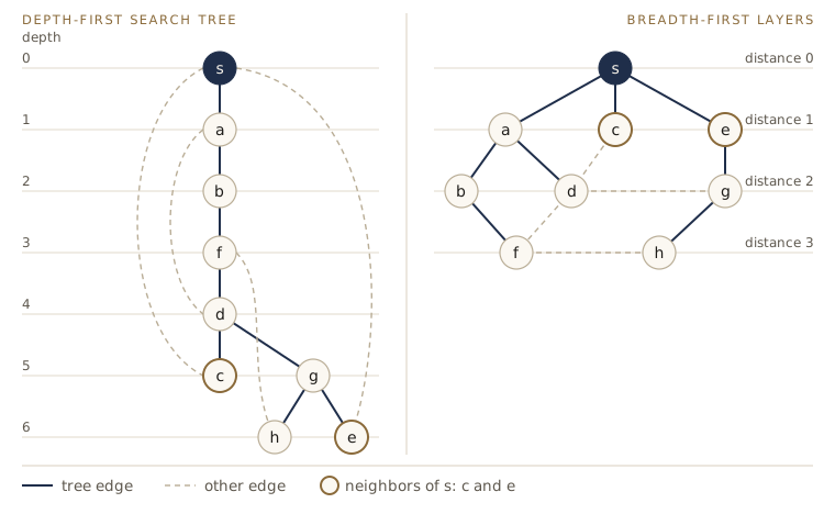
s. Solid navy lines are tree edges, dashed lines are the other edges. The DFS tree (left) reaches c and e at depths 5 and 6; the BFS layers (right) put every vertex at its distance from s.Breadth-first search
The idea: layer by layer
Group the vertices by their distance from \(s\) into layers: layer 0 is \(\{s\}\), layer 1 the vertices at distance 1, and so on. Suppose we already know layers \(0, 1, \dots, d\). Which vertices are in layer \(d + 1\)? Exactly those that are not in any earlier layer but have an edge from some vertex in layer \(d\). So one layer determines the next, and we can compute them in order.
Breadth-first search (BFS) carries this out with a queue, a list with first-in, first-out order: we inject at the back and eject from the front. The queue starts with \(s\). Each time we eject a vertex \(u\), we look at its neighbors; every neighbor we have not seen before gets distance \(\text{dist}(u) + 1\), a prev pointer to \(u\), and a place at the back of the queue. Because vertices of layer \(d\) enter the queue before any vertex of layer \(d + 1\), the queue processes the layers in order. Python’s collections.deque gives a queue with constant-time operations at both ends.
def bfs(G, s, trace=False):
    """Breadth-first search from s in an unweighted graph {u: [v, ...]}.
    Returns (dist, prev): dist[v] = number of edges on a shortest path from s to v
    (INF if unreachable), prev[v] = the vertex before v on that path."""
    dist = {u: INF for u in G}
    prev = {u: None for u in G}
    dist[s] = 0
    Q = deque([s])
    while Q:
        u = Q.popleft()                  # eject from the front
        for v in G[u]:
            if dist[v] == INF:           # first time we see v
                dist[v] = dist[u] + 1
                prev[v] = u
                Q.append(v)              # inject at the back
        if trace:
            print(f"eject {u}   queue now: {' '.join(Q) or '(empty)'}")
    return dist, prev

dist, prev = bfs(G, "s", trace=True)
eject s   queue now: a c e
eject a   queue now: c e b d
eject c   queue now: e b d
eject e   queue now: b d g
eject b   queue now: d g f
eject d   queue now: g f
eject g   queue now: f h
eject f   queue now: h
eject h   queue now: (empty)
Watch the queue: after s is ejected it holds exactly layer 1 (a c e); once those three are ejected it holds exactly layer 2 (b d g); then layer 3 (f h). Grouping the vertices by dist shows the layers directly, and the prev pointers now give short paths.
def layers(dist):
    """Group the reachable vertices by distance."""
    out = {}
    for v, d in dist.items():
        if d < INF:
            out.setdefault(d, []).append(v)
    return [sorted(out[d]) for d in sorted(out)]

print(layers(dist))
for t in ["c", "e", "h"]:
    print(f"BFS path to {t}: {' -> '.join(path_to(prev, t))}   (dist {dist[t]})")
[['s'], ['a', 'c', 'e'], ['b', 'd', 'g'], ['f', 'h']]
BFS path to c: s -> c   (dist 1)
BFS path to e: s -> e   (dist 1)
BFS path to h: s -> e -> g -> h   (dist 3)
The edges \((\text{prev}(v), v)\) form a tree rooted at \(s\) — every vertex except \(s\) has exactly one parent, and parents are discovered before their children — and every path in it from \(s\) is a shortest path. A tree with that property is a shortest-path tree. It is a compact answer to the whole single-source problem: \(\lvert V \rvert - 1\) pointers encode a shortest path to every reachable vertex, and path_to reads any one of them off in time proportional to its length.
Note. BFS is almost the same code as the iterative, stack-based version of DFS: swap the stack for a queue and the search changes character. DFS plunges deep and backs up only when stuck; BFS spreads out evenly, like a ripple, visiting vertices in order of distance. Note also that BFS does not restart from other vertices when the queue empties: vertices not reachable from \(s\) keep distance \(\infty\), which is the right answer.
Correctness
Write \(L_d\) for the set of vertices at distance exactly \(d\) from \(s\).
Lemma (BFS). For every \(d \ge 0\) with \(L_d\) nonempty, there is a moment during BFS at which (1) every vertex at distance at most \(d\) has its correct
dist, (2) every other vertex still hasdistequal to \(\infty\), and (3) the queue contains exactly the vertices of \(L_d\).
The idea is that processing one complete layer discovers exactly the next layer. Formally, we argue by induction on \(d\). For \(d = 0\) the moment is the start: only \(s\) has a finite distance, it is correct, and the queue is \([s]\).
Now assume the statement for \(d\), and consider what happens while the vertices of \(L_d\) are ejected one by one. Take any \(u \in L_d\) and a neighbor \(v\) with \(\text{dist}(v) = \infty\). By (1) and (2), \(v\) is not at distance \(\le d\); the edge from \(u\) gives a path of length \(d + 1\); so \(v \in L_{d+1}\), and BFS sets \(\text{dist}(v) = d + 1\), which is correct. Conversely, every \(w \in L_{d+1}\) has a shortest path whose second-to-last vertex is in \(L_d\), so \(w\) is discovered when that vertex is ejected (if not earlier in the same phase). No vertex outside \(L_{d+1}\) is discovered, because every newly discovered vertex was just shown to lie in \(L_{d+1}\). So when the last vertex of \(L_d\) has been ejected, the queue holds exactly \(L_{d+1}\), the vertices at distance \(\le d + 1\) have correct distances, and all others are still at \(\infty\). That is the statement for \(d + 1\).
Every reachable vertex lies in some layer, so every reachable vertex gets its correct distance, and unreachable ones stay at \(\infty\). For the prev pointers: when \(v \in L_{d+1}\) is discovered from \(u \in L_d\), the path to \(u\) in the tree (of length \(d\), by induction) followed by the edge \((u, v)\) has length \(d + 1 = d(s, v)\).
A proof is the real guarantee, but a test catches slips in the code. For tiny graphs we can find distances by brute force: try every simple path out of \(s\) and keep the shortest length to each vertex. (A shortest path never repeats a vertex, since cutting out the loop between two visits makes it shorter.) This takes exponential time, which is fine for seven vertices.
def brute_force_hops(G, s):
    """Fewest edges from s to each vertex, by trying every simple path. Exponential time."""
    best = {u: INF for u in G}
    def extend(u, hops, on_path):
        best[u] = min(best[u], hops)
        for v in G[u]:
            if v not in on_path:
                on_path.add(v)
                extend(v, hops + 1, on_path)
                on_path.remove(v)
    extend(s, 0, {s})
    return best

def random_digraph(n, m, rng):
    """A directed graph on vertices 0..n-1 with m distinct edges chosen at random."""
    pairs = [(u, v) for u in range(n) for v in range(n) if u != v]
    G = {u: [] for u in range(n)}
    for u, v in rng.sample(pairs, m):
        G[u].append(v)
    return G

rng = random.Random(1)
trials = 500
agree = 0
for _ in range(trials):
    n = rng.randint(2, 7)
    H = random_digraph(n, rng.randint(0, n * (n - 1)), rng)
    agree += bfs(H, 0)[0] == brute_force_hops(H, 0)
print(f"BFS agrees with brute force on {agree} of {trials} random directed graphs")
BFS agrees with brute force on 500 of 500 random directed graphs
Running time
BFS runs in \(O(\lvert V \rvert + \lvert E \rvert)\) time, for the same reasons as DFS. Initializing dist and prev takes \(O(\lvert V \rvert)\). A vertex enters the queue only when its dist changes from \(\infty\), which happens at most once, so there are at most \(\lvert V \rvert\) injects and \(\lvert V \rvert\) ejects, each \(O(1)\). When \(u\) is ejected, the inner loop scans its adjacency list once, so over the whole run the inner loop does \(\sum_u \deg(u)\) iterations: \(\lvert E \rvert\) in a directed graph, \(2\lvert E \rvert\) in an undirected one. Each iteration is constant work.
Lengths on edges
BFS counts edges, but in most applications edges are not all alike. A road between two towns has a length in miles or a driving time in minutes; a network link has a delay; a flight has a price. From now on each edge \(e = (u, v)\) carries a number \(\ell(u, v)\), its length (or weight; the two words mean the same here). The length of a path is the sum of the lengths of its edges, and distance and shortest path are defined as before with this new length. Lengths need not be physical distances — anything additive that we want to minimize will do — and in the Bellman–Ford section we will even allow negative ones. Until then, assume every length is positive.
In code a weighted graph is {u: [(v, w), ...]}. Here is a small directed example. BFS, which ignores the weights, finds the path with the fewest edges — which is not the shortest one.
W = {
    "s": [("a", 4), ("b", 1)],
    "a": [("c", 1), ("d", 5)],
    "b": [("a", 2), ("c", 6), ("e", 7)],
    "c": [("d", 2), ("e", 3)],
    "d": [("f", 2)],
    "e": [("f", 2)],
    "f": [],
}

def unweighted(G):
    """Drop the lengths: {u: [(v, w), ...]} -> {u: [v, ...]}."""
    return {u: [v for v, _ in G[u]] for u in G}

def path_length(G, path):
    """Total length of a path given as a list of vertices."""
    return sum(dict(G[u])[v] for u, v in zip(path, path[1:]))

_, prev_bfs = bfs(unweighted(W), "s")
p = path_to(prev_bfs, "d")
print("fewest edges:", " -> ".join(p), "  length", path_length(W, p))
q = ["s", "b", "a", "c", "d"]
print("a better one:", " -> ".join(q), "  length", path_length(W, q))
fewest edges: s -> a -> d   length 9
a better one: s -> b -> a -> c -> d   length 6
Splitting edges into unit pieces
If every length is a positive integer, there is an easy reduction to the unweighted case. Replace each edge \((u, v)\) of length \(\ell\) by a chain of \(\ell\) unit edges through \(\ell - 1\) new dummy vertices. Distances between the original vertices do not change — a path of length \(\ell\) in the old graph becomes a path of \(\ell\) edges in the new one, and vice versa — and now BFS applies.
def subdivide(G):
    """Replace each edge of integer length w by a chain of w unit edges.
    Dummy vertices are tuples (u, v, i) and never clash with the original names."""
    H = {u: [] for u in G}
    for u in G:
        for v, w in G[u]:
            chain = [u] + [(u, v, i) for i in range(1, w)] + [v]
            for x, y in zip(chain, chain[1:]):
                H.setdefault(x, []).append(y)
    return H

W_split = subdivide(W)
dist_split, _ = bfs(W_split, "s")
print(len(W), "vertices became", len(W_split))
print({v: dist_split[v] for v in W})
7 vertices became 31
{'s': 0, 'a': 3, 'b': 1, 'c': 4, 'd': 6, 'e': 7, 'f': 8}
These are the true distances (we will confirm them in a moment by a second method). But the reduction is only practical when lengths are small: the new graph has \(\lvert V \rvert + \sum_e (\ell_e - 1)\) vertices, so an edge of length one million contributes a million dummy vertices, and BFS spends nearly all its time crawling along chains toward vertices nobody asked about.
Alarm clocks
We can keep the idea and drop the waste. Picture BFS on the subdivided graph as a wavefront advancing one unit of length per minute from \(s\). Between the moments when the wavefront reaches an original vertex, nothing of interest happens: it is moving along the interior of some chains. So instead of watching minute by minute, set an alarm for each original vertex at the time the front is expected to arrive there, and sleep until the next alarm.
- At time 0, set an alarm for \(s\).
- Repeat until no alarms are left: let the next alarm go off, at time \(T\), for vertex \(u\). Then \(d(s, u) = T\). For each edge \((u, v)\) out of \(u\), the front will now also reach \(v\) at time \(T + \ell(u, v)\). If \(v\) has no alarm yet, set one for that time; if its alarm is set for later, move it earlier.
An alarm can be an overestimate — a faster route to \(v\) may be discovered later, as the front reaches other vertices — which is why alarms can be moved. But no alarm can go off too early, and nothing happens between alarms, so each alarm marks the true arrival time of the front. Here is the simulation, on a graph whose long edges would make the subdivided version huge.
def alarm_clock(G, s, trace=False):
    """Simulate BFS on the subdivided graph, waking only when the
    front reaches a real vertex."""
    alarms = {s: 0}  # vertex -> time its alarm is set for
    dist = {}
    while alarms:
        u = min(alarms, key=alarms.get)         # the next alarm to go off
        T = alarms.pop(u)
        dist[u] = T
        notes = []
        for v, w in G[u]:
            if v in dist:
                continue
            if v not in alarms:
                alarms[v] = T + w
                notes.append(f"set {v} for {T + w}")
            elif T + w < alarms[v]:
                notes.append(f"move {v} from {alarms[v]} to {T + w}")
                alarms[v] = T + w
        if trace:
            print(f"T = {T:3}: reached {u}   " + "; ".join(notes))
    return dist

X = {"s": [("a", 70), ("b", 180)],
     "a": [("b", 60), ("c", 90)],
     "b": [("c", 10)],
     "c": []}
alarm_clock(X, "s", trace=True)
print("subdividing X would create", len(subdivide(X)) - len(X), "dummy vertices")
T =   0: reached s   set a for 70; set b for 180
T =  70: reached a   move b from 180 to 130; set c for 160
T = 130: reached b   move c from 160 to 140
T = 140: reached c
subdividing X would create 405 dummy vertices
Four wake-ups instead of 140 minutes of watching 409 vertices. On W the alarm clock reproduces the BFS-on-chains distances exactly:
alarm_clock(W, "s") == {v: dist_split[v] for v in W}
True
All that remains is a good way to keep track of the alarms. The simulation above finds the next alarm by scanning all of them, which is slow when there are many. That bookkeeping problem, and its solution, is Dijkstra’s algorithm.
Dijkstra’s algorithm
From alarms to a priority queue
The alarm clock needs a data structure that holds a set of elements (vertices), each with a numeric key (its alarm time), and supports:
- insert: add a new element with a given key;
- decrease-key: lower the key of an element already in the set;
- delete-min: remove and return the element with the smallest key.
Such a structure is a priority queue. Some implementations also offer make-queue, which builds a priority queue from many elements at once, often faster than inserting them one at a time. With a priority queue, the alarm clock becomes Dijkstra’s algorithm: dist[v] is the current alarm setting for \(v\) (\(\infty\) if none is set), delete-min tells us whose alarm goes off next, and insert or decrease-key sets or moves an alarm. Like BFS, it keeps a prev pointer for each vertex: the vertex whose edge last lowered its dist.
One way to put it: Dijkstra’s algorithm is BFS with the queue replaced by a priority queue, so that vertices come out in order of their distance measured by edge lengths rather than by edge counts.
The code, with Python’s heapq
Python’s standard library has a priority queue in the module heapq, a binary heap stored in a plain list (we build our own binary heap in the next section). It supports insert (heappush) and delete-min (heappop), but not decrease-key. The standard workaround is lazy deletion: to decrease the key of \(v\), push a new entry (new_dist, v) and leave the old one in the heap. The new entry has the smaller key, so it comes out first; when the old one comes out later, \(v\) is already finished and we skip it as stale.
def dijkstra(G, s, trace=False, stats=None):
    """Dijkstra's algorithm on {u: [(v, w), ...]} with non-negative lengths w.
    Returns (dist, prev). A binary heap (heapq) with lazy deletion
    stands in for decrease-key."""
    dist = {u: INF for u in G}
    prev = {u: None for u in G}
    dist[s] = 0
    heap = [(0, s)]                      # entries (tentative distance, vertex)
    done = set()                         # vertices whose distance is final
    pushes, pops = 1, 0
    while heap:
        d, u = heapq.heappop(heap)       # delete-min
        pops += 1
        if u in done:  # stale: u is already finished
            if trace:
                print(f"pop {u} ({d})  stale, skip")
            continue
        done.add(u)
        changes = []
        for v, w in G[u]:
            if dist[u] + w < dist[v]:
                changes.append(f"{v}: {dist[v]} -> {dist[u] + w}")
                dist[v] = dist[u] + w
                prev[v] = u
                heapq.heappush(heap, (dist[v], v))     # insert, or "decrease-key"
                pushes += 1
        if trace:
            print(f"pop {u} ({d})  " + ("; ".join(changes) or "no updates"))
    if stats is not None:
        stats.update(pushes=pushes, pops=pops, finished=len(done))
    return dist, prev

dist, prev = dijkstra(W, "s", trace=True)
pop s (0)  a: inf -> 4; b: inf -> 1
pop b (1)  a: 4 -> 3; c: inf -> 7; e: inf -> 8
pop a (3)  c: 7 -> 4; d: inf -> 8
pop a (4)  stale, skip
pop c (4)  d: 8 -> 6; e: 8 -> 7
pop d (6)  f: inf -> 8
pop c (7)  stale, skip
pop e (7)  no updates
pop d (8)  stale, skip
pop e (8)  stale, skip
pop f (8)  no updates
Read the trace as the alarm clock. At the start only s has an alarm. When s is popped, a and b get alarms at 4 and 1. Popping b moves a’s alarm from 4 to 3 — the route through b is quicker than the direct edge — and so on. The vertices are finished in the order s, b, a, c, d, e, f, with distances 0, 1, 3, 4, 6, 7, 8, which never decrease. Four pops are stale: they are the leftover entries of keys that were later lowered.
print(dist)
for t in ["d", "f"]:
    print(f"shortest path to {t}: {' -> '.join(path_to(prev, t))}   (length {dist[t]})")
{'s': 0, 'a': 3, 'b': 1, 'c': 4, 'd': 6, 'e': 7, 'f': 8}
shortest path to d: s -> b -> a -> c -> d   (length 6)
shortest path to f: s -> b -> a -> c -> d -> f   (length 8)
The distances match the subdivided BFS above.
Note. Lazy deletion changes the heap’s size, not the algorithm. Each successful update pushes one entry, so the heap holds at most \(\lvert E \rvert + 1\) entries instead of at most \(\lvert V \rvert\). Since \(\lvert E \rvert \le \lvert V \rvert^2\), each heap operation still costs \(O(\log \lvert E \rvert) = O(\log \lvert V \rvert)\), so the running-time bound below is unchanged; the price is \(O(\lvert E \rvert)\) extra memory. Ties among entries with equal keys are broken by comparing vertex names, so the names in one graph must be mutually comparable (all strings, or all integers).
Correctness: the known region
The alarm-clock story explains why Dijkstra’s algorithm should work, but it depends on the subdivision, which needs integer lengths. Here is a direct argument that works for any non-negative real lengths. It views the algorithm as growing a known region \(R\) — the set of finished vertices, done in the code — outward from \(s\), always adding the vertex outside \(R\) that is closest to \(s\).
Call a path from \(s\) an \(R\)-path if all its vertices except possibly the last one lie in \(R\). The heart of the argument is a claim about what dist means while the algorithm runs.
Theorem (Dijkstra). If all edge lengths are non-negative, then whenever a vertex is added to the known region \(R\): (1) for every \(u \in R\), \(\text{dist}(u) = d(s, u)\); and (2) for every \(v \notin R\), \(\text{dist}(v)\) is the length of a shortest \(R\)-path from \(s\) to \(v\) (\(\infty\) if there is none). In particular every vertex receives its true distance.
The idea is that the closest vertex outside the region can be reached by stepping out of the region once, so the best one-step extension is a genuine shortest path. We argue by induction on the number of vertices in \(R\). Before the first vertex is added, \(R\) is empty; the only \(R\)-path is the one-vertex path \(s\), and indeed \(\text{dist}(s) = 0\) and every other dist is \(\infty\).
Suppose (1) and (2) hold, and the algorithm next adds \(v\), the vertex outside \(R\) with the smallest dist. Take any path \(P\) from \(s\) to \(v\), and let \(y\) be the first vertex of \(P\) that is not in \(R\) (there is one, since \(v \notin R\)). The part of \(P\) up to \(y\) is an \(R\)-path to \(y\), so by (2) its length is at least \(\text{dist}(y)\), which is at least \(\text{dist}(v)\) by the choice of \(v\). The rest of \(P\), from \(y\) to \(v\), has non-negative length. So every path to \(v\) has length at least \(\text{dist}(v)\), and by (2) some \(R\)-path achieves it: \(\text{dist}(v) = d(s, v)\). That is (1) for the enlarged region.
For (2), consider a vertex \(z\) still outside the enlarged region \(R' = R \cup \{v\}\). A shortest \(R'\)-path to \(z\) either avoids \(v\) — then it is an \(R\)-path, of length \(\text{dist}(z)\) already — or it passes through \(v\). If \(v\) is not its second-to-last vertex, the path goes on from \(v\) to some \(x \in R\); but \(d(s, x) \le d(s, v)\), so replacing the part up to \(x\) by a shortest path to \(x\) inside \(R\) gives an \(R'\)-path to \(z\) that is no longer. So we may assume the path ends \(\dots \to v \to z\), with length \(d(s, v) + \ell(v, z)\). That is exactly the value the loop over the edges out of \(v\) compares against \(\text{dist}(z)\), keeping the smaller. This proves (2).
(With lazy deletion the heap may also contain stale entries, but the algorithm skips them, so the vertex it adds is still the one outside \(R\) with the smallest dist.)
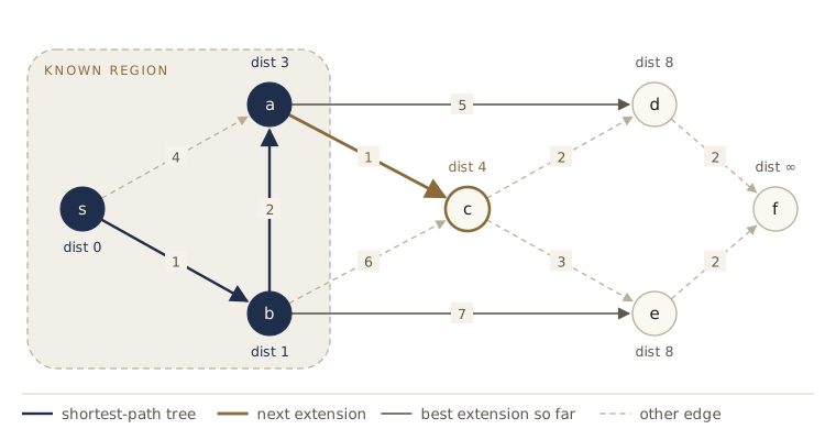
W after three vertices are finished. Tentative distances outside the known region are the lengths of the best one-edge extensions of known shortest paths. The smallest, 4 via a → c, is a true distance, so c joins the region next.The proof also shows what the prev pointers are. When \(\text{dist}(v)\) is set for the last time, it is set by an edge \((u, v)\) with \(u\) already finished and \(\text{dist}(v) = d(s, u) + \ell(u, v)\), so following prev pointers from \(v\) traces a shortest path, and together they form a shortest-path tree.
Running time
Count the work in terms of priority-queue operations. Each reachable vertex is inserted once and removed by delete-min once. Each edge \((u, v)\) is examined once, when \(u\) is removed, and causes at most one insert or decrease-key. So Dijkstra’s algorithm performs
\[\lvert V \rvert \text{ delete-mins} \quad\text{and}\quad \text{at most } \lvert V \rvert + \lvert E \rvert \text{ inserts and decrease-keys},\]plus \(O(\lvert V \rvert + \lvert E \rvert)\) other work, exactly as in BFS. The total time is therefore
\[O\big(\lvert V \rvert \cdot t_{\text{deletemin}} + (\lvert V \rvert + \lvert E \rvert) \cdot t_{\text{insert}} \big),\]and it depends on how fast the priority queue is. With a binary heap each operation is \(O(\log \lvert V \rvert)\) and the total is \(O((\lvert V \rvert + \lvert E \rvert) \log \lvert V \rvert)\). With lazy deletion every successful update is one push, and every push is eventually popped, so pushes and pops are both at most \(\lvert E \rvert + 1\). Let’s count them on random graphs.
def random_weighted(n, m, rng, lo=1, hi=9):
    """A directed graph on 0..n-1 with m distinct edges and random
    integer lengths in [lo, hi]."""
    G = random_digraph(n, m, rng)
    return {u: [(v, rng.randint(lo, hi)) for v in G[u]] for u in G}

rng = random.Random(2)
for n, m in [(1_000, 4_000), (1_000, 40_000), (300, 300 * 299)]:
    H = random_weighted(n, m, rng, 1, 1000)
    stats = {}
    dijkstra(H, 0, stats=stats)
    print(f"V = {n:5,}  E = {m:6,}   pushes = pops = {stats['pops']:5,}"
          f"   stale = {stats['pops'] - stats['finished']:5,}   V + E + 1 = {n + m + 1:6,}")
V = 1,000  E =  4,000   pushes = pops = 1,266   stale =   289   V + E + 1 =  5,001
V = 1,000  E = 40,000   pushes = pops = 3,238   stale = 2,238   V + E + 1 = 41,001
V =   300  E = 89,700   pushes = pops = 1,524   stale = 1,224   V + E + 1 = 90,001
Two things to notice. First, the counts respect the bound. Second, on random lengths they are far below it: most edges fail to improve anything, because by the time an edge \((u, v)\) is examined, \(v\) usually already has a good tentative distance. The worst case bound is reached only on graphs built so that every edge improves a distance (exercise 5 asks you to build one); the analysis has to allow for them.
Negative edges break it
The proof used non-negative lengths in exactly one place: the part of path \(P\) after it leaves the region cannot be negative. With a negative edge, a path can wander out of the region, grow long, and then come back cheaply. Here is a four-vertex example.
NEG_SMALL = {"s": [("a", 2), ("b", 4)],
             "a": [("c", 1)],
             "b": [("a", -3)],
             "c": []}
dist, prev = dijkstra(NEG_SMALL, "s", trace=True)
print(dist)
pop s (0)  a: inf -> 2; b: inf -> 4
pop a (2)  c: inf -> 3
pop c (3)  no updates
pop b (4)  a: 2 -> 1
pop a (1)  stale, skip
{'s': 0, 'a': 1, 'b': 4, 'c': 3}
The algorithm finished a at distance 2 and c at 3. Only later did it discover the route s -> b -> a of length \(4 - 3 = 1\), and by then c was finished: the true distance to c is 2, not 3. The algorithm even lowered dist(a) to 1 after a was finished, but that change never reached c. The Bellman–Ford algorithm below handles such graphs.
Watch out. Dijkstra’s algorithm requires non-negative edge lengths. With a negative edge it can return wrong distances without any sign of trouble. Adding a large constant to every edge to make it non-negative does not help: it penalizes paths with many edges more than paths with few, so it can change which path is shortest.
Priority queue implementations
Dijkstra’s algorithm is as fast as its priority queue. We look at three implementations and at how the choice interacts with the shape of the graph.
An unordered array
The simplest priority queue is an unordered table of keys, one entry per element. Insert and decrease-key just write a key: \(O(1)\). Delete-min must scan every remaining key: \(O(n)\) for \(n\) elements. The alarm-clock code above is exactly this implementation (min(alarms, key=alarms.get) is the scan). In Dijkstra’s algorithm it gives \(\lvert V \rvert\) scans of \(O(\lvert V \rvert)\) each plus \(O(\lvert E \rvert)\) constant-time updates: \(O(\lvert V \rvert^2)\) in total. We write it as a class so that it can be swapped for the heaps below; it counts its operations and key comparisons.
class ArrayPQ:
    """Priority queue as an unordered table of keys:
    O(1) insert and decrease-key, O(n) delete-min."""
    def __init__(self):
        self.key = {}
        self.ops = {"insert": 0, "decrease_key": 0, "delete_min": 0}
        self.comparisons = 0

    def __len__(self):
        return len(self.key)

    def insert(self, x, k):
        self.ops["insert"] += 1
        self.key[x] = k

    def decrease_key(self, x, k):
        self.ops["decrease_key"] += 1
        self.key[x] = k

    def delete_min(self):
        self.ops["delete_min"] += 1
        items = iter(self.key)
        best = next(items)
        for x in items:                      # scan every remaining element
            self.comparisons += 1
            if self.key[x] < self.key[best]:
                best = x
        return best, self.key.pop(best)
Binary heaps
A binary heap stores the elements in a complete binary tree: every level is full except possibly the last, which is filled from the left. The keys satisfy the heap property: every node’s key is at most the keys of its children. So the smallest key is always at the root. A complete tree with \(n\) nodes has height \(\lfloor \log_2 n \rfloor\), and every operation walks along one root-to-leaf path:
- insert: put the new element in the first free position of the bottom level, then let it bubble up: while it is smaller than its parent, swap the two. At most one swap per level.
- decrease-key: lower the key and bubble the element up from where it is.
- delete-min: the answer is at the root. Move the last element of the bottom level into the root, then let it sift down: while it is larger than its smaller child, swap it with that child.
Each of these takes \(O(\log n)\) time. Because the tree is complete, it needs no pointers: number the nodes level by level, left to right, starting from 1 at the root, and store node \(j\) at index \(j\) of a list. Then the parent of node \(j\) is node \(\lfloor j/2 \rfloor\), and its children are nodes \(2j\) and \(2j + 1\) (when they exist).
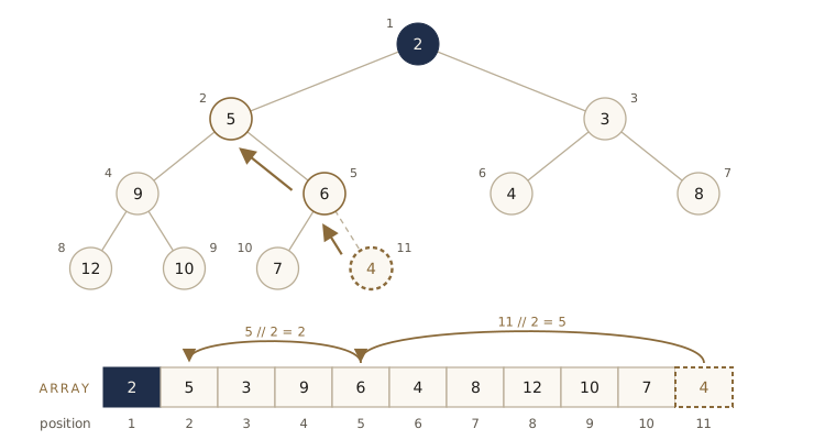
For decrease-key the heap must find an element’s position quickly, so the class keeps a second dict, pos, from element to index, and updates it on every swap. Everything that depends on the shape of the tree is in the two small methods parent and children; we will override just those to get d-ary heaps.
class BinaryHeap:
    """Min-priority queue of distinct elements with numeric keys.
    The tree is stored in self.h[1..n] (slot 0 is unused), so node j has parent j // 2
    and children 2j, 2j + 1. self.pos[x] is x's index in self.h, needed for decrease_key."""
    def __init__(self):
        self.h = [None]
        self.key = {}
        self.pos = {}
        self.ops = {"insert": 0, "decrease_key": 0, "delete_min": 0}
        self.comparisons = 0

    def __len__(self):
        return len(self.h) - 1

    # the shape of the tree
    def parent(self, j):
        return j // 2

    def children(self, j):
        return range(2 * j, min(2 * j + 1, len(self)) + 1)

    # helpers
    def _smaller(self, i, j):
        """Is the key at position i smaller than the key at position j?"""
        self.comparisons += 1
        return self.key[self.h[i]] < self.key[self.h[j]]

    def _swap(self, i, j):
        h = self.h
        h[i], h[j] = h[j], h[i]
        self.pos[h[i]], self.pos[h[j]] = i, j

    def _bubble_up(self, j):
        while j > 1 and self._smaller(j, self.parent(j)):
            self._swap(j, self.parent(j))
            j = self.parent(j)

    def _sift_down(self, j):
        while True:
            kids = self.children(j)
            if not kids:
                return
            c = kids[0]  # find the child with the smallest key
            for k in kids[1:]:
                if self._smaller(k, c):
                    c = k
            if not self._smaller(c, j):
                return
            self._swap(j, c)
            j = c

    # the priority-queue operations
    def insert(self, x, k):
        self.ops["insert"] += 1
        self.key[x] = k
        self.h.append(x)
        self.pos[x] = len(self)
        self._bubble_up(len(self))

    def decrease_key(self, x, k):
        self.ops["decrease_key"] += 1
        assert k <= self.key[x], "decrease_key cannot raise a key"
        self.key[x] = k
        self._bubble_up(self.pos[x])

    def delete_min(self):
        self.ops["delete_min"] += 1
        top = self.h[1]
        self._swap(1, len(self))  # move the last element to the root
        self.h.pop()
        del self.pos[top]
        k = self.key.pop(top)
        if len(self) > 0:
            self._sift_down(1)
        return top, k

    @classmethod
    def from_keys(cls, keys, **kwargs):
        """make-queue: build a heap from a dict {element: key} bottom-up, in O(n) time."""
        heap = cls(**kwargs)
        for x, k in keys.items():
            heap.key[x] = k
            heap.h.append(x)
            heap.pos[x] = len(heap)
        for j in range(len(heap) // 2, 0, -1):  # internal nodes, last first
            heap._sift_down(j)
        return heap

    def keys(self):
        """The keys in array order, for display."""
        return [self.key[x] for x in self.h[1:]]
Let’s replay the figure. The ten keys below already satisfy the heap property, so from_keys leaves them in place. Inserting key 4 bubbles it up to position 2; then delete-min removes the root, moves the last element (key 6) to the top, and sifts it down.
H = BinaryHeap.from_keys(dict(zip("abcdefghij", [2, 5, 3, 9, 6, 4, 8, 12, 10, 7])))
print("heap:          ", H.keys())
H.insert("k", 4)
print("insert 4:      ", H.keys(), "  now at position", H.pos["k"])
print("delete-min ->  ", H.delete_min(), " leaves", H.keys())
heap:           [2, 5, 3, 9, 6, 4, 8, 12, 10, 7]
insert 4:       [2, 4, 3, 9, 5, 4, 8, 12, 10, 7, 6]   now at position 2
delete-min ->   ('a', 2)  leaves [3, 4, 4, 9, 5, 6, 8, 12, 10, 7]
A data structure with this many index calculations deserves a test. We run random sequences of inserts, decrease-keys, and delete-mins, compare every delete-min with a plain dict that finds the minimum by brute force, and check the heap property and the pos table after every step.
def check_heap(H):
    """The heap property holds and pos agrees with the array."""
    n = len(H)
    assert all(H.key[H.h[H.parent(j)]] <= H.key[H.h[j]] for j in range(2, n + 1))
    assert all(H.pos[H.h[j]] == j for j in range(1, n + 1)) and len(H.pos) == n

def random_heap_test(make_heap, trials, steps, rng):
    ops_done = 0
    for _ in range(trials):
        H, ref, fresh = make_heap(), {}, 0
        for _ in range(steps):
            r = rng.random()
            if r < 0.45 or not ref:                        # insert a new element
                ref[fresh] = rng.randint(0, 99)
                H.insert(fresh, ref[fresh])
                fresh += 1
            elif r < 0.75:  # decrease a key
                x = rng.choice(list(ref))
                ref[x] -= rng.randint(0, 30)
                H.decrease_key(x, ref[x])
            else:                                          # delete-min
                x, k = H.delete_min()
                assert k == min(ref.values()) and ref.pop(x) == k
            check_heap(H)
            ops_done += 1
    return ops_done

rng = random.Random(3)
print(random_heap_test(BinaryHeap, 300, 60, rng), "random operations, all checks passed")
18000 random operations, all checks passed
Now Dijkstra’s algorithm with a real decrease-key. This is the textbook form: a vertex is inserted when it first gets a finite distance, and its key is decreased when a shorter route turns up. With non-negative lengths a finished vertex never has its dist lowered again, so decrease-key is only ever called on vertices still in the queue.
def dijkstra_pq(G, s, pq):
    """Dijkstra's algorithm with an explicit priority queue pq
    (an ArrayPQ, a BinaryHeap, ...)."""
    dist = {u: INF for u in G}
    prev = {u: None for u in G}
    dist[s] = 0
    pq.insert(s, 0)
    while len(pq) > 0:
        u, du = pq.delete_min()
        for v, w in G[u]:
            if du + w < dist[v]:
                if dist[v] == INF:
                    pq.insert(v, du + w)
                else:
                    pq.decrease_key(v, du + w)
                dist[v] = du + w
                prev[v] = u
    return dist, prev

for pq in [ArrayPQ(), BinaryHeap()]:
    dist_pq, _ = dijkstra_pq(W, "s", pq)
    print(type(pq).__name__, dist_pq == dijkstra(W, "s")[0], pq.ops)
ArrayPQ True {'insert': 7, 'decrease_key': 4, 'delete_min': 7}
BinaryHeap True {'insert': 7, 'decrease_key': 4, 'delete_min': 7}
Both queues give the same distances as the heapq version. On W there are 7 inserts and 7 delete-mins, one of each per vertex, and 4 decrease-keys: the four times an alarm was moved in the trace (a from 4 to 3, c from 7 to 4, d from 8 to 6, e from 8 to 7). That is 7 + 4 = 11 inserts and decrease-keys, one for each of the 11 successful updates, which matches the 11 pushes of the lazy version.
Building a heap in linear time
The from_keys method is the make-queue operation. Instead of \(n\) inserts, which cost up to \(O(n \log n)\), it places all elements in the array in any order and then sifts down every internal node, starting from the last one and moving toward the root. When node \(j\) is sifted down, both of its subtrees are already heaps, so afterward the subtree rooted at \(j\) is a heap. A node at height \(h\) costs \(O(h)\), and a complete tree has only about \(n / 2^{h+1}\) nodes at height \(h\), so the total is
since \(\sum_h h/2^{h+1} = 1\). The comparison counts agree: at most about \(2n\), even for the worst ordering.
for n in [1_000, 10_000, 100_000]:
    H = BinaryHeap.from_keys({i: n - i for i in range(n)})   # reverse order
    check_heap(H)
    c = H.comparisons
    print(f"n = {n:7,}   comparisons = {c:7,}   per element = {c / n:.2f}")
n =   1,000   comparisons =   1,982   per element = 1.98
n =  10,000   comparisons =  19,982   per element = 2.00
n = 100,000   comparisons = 199,978   per element = 2.00
d-ary heaps
A d-ary heap is the same structure with \(d\) children per node instead of two. In the 1-indexed array, node \(j\) has parent \(\lfloor (j - 2)/d \rfloor + 1\) and children \((j-1)d + 2\) through \((j - 1)d + d + 1\); for \(d = 2\) these are the familiar \(\lfloor j/2 \rfloor\), \(2j\), and \(2j + 1\). The tree is flatter: its height is about \(\log_d n = \log n / \log d\). That makes insert and decrease-key faster, \(O(\log n / \log d)\), since bubbling up does one comparison per level. Delete-min gets slower, \(O(d \log n / \log d)\), because sifting down must find the smallest of \(d\) children at every level.
class DaryHeap(BinaryHeap):
    """A heap in which every node has up to d children."""
    def __init__(self, d=4):
        super().__init__()
        self.d = d

    def parent(self, j):
        return (j - 2) // self.d + 1

    def children(self, j):
        first = (j - 1) * self.d + 2
        return range(first, min(first + self.d - 1, len(self)) + 1)

rng = random.Random(4)
for d in [3, 4, 7]:
    done = random_heap_test(lambda: DaryHeap(d), 100, 60, rng)
    print(f"d = {d}: {done} random operations, all checks passed")
d = 3: 6000 random operations, all checks passed
d = 4: 6000 random operations, all checks passed
d = 7: 6000 random operations, all checks passed
To see the trade-off, insert \(n = 4095\) keys in decreasing order, so that every insert bubbles all the way to the root, then delete them all, and count comparisons per operation.
n = 4095
print(" d    height   comparisons per insert   per delete-min")
for d in [2, 4, 8, 16]:
    H = DaryHeap(d)
    for i in range(n):
        H.insert(i, n - i)                   # each new key is the smallest so far
    per_insert = H.comparisons / n
    height = math.floor(math.log(n * (d - 1) + 1, d) - 1e-9)
    H.comparisons = 0
    for _ in range(n):
        H.delete_min()
    print(f"{d:2}    {height:4}   {per_insert:20.1f}   {H.comparisons / n:14.1f}")
 d    height   comparisons per insert   per delete-min
 2      11                   10.0             18.5
 4       6                    5.6             19.7
 8       4                    3.8             26.2
16       3                    2.9             38.4
Inserts get cheaper as \(d\) grows, in step with the height \(\log_d n\): each one here climbs the whole tree, one comparison per level. Delete-mins get more expensive, roughly like \(d \log_d n\), because each level of the sift-down compares \(d\) keys. That asymmetry is useful: Dijkstra’s algorithm can do up to \(\lvert E \rvert\) decrease-keys but only \(\lvert V \rvert\) delete-mins, so on a graph with many edges per vertex it pays to make decrease-key cheap at the expense of delete-min.
Which priority queue is best?
Plugging the operation costs into the count \(\lvert V \rvert\) delete-mins and \(\lvert V \rvert + \lvert E \rvert\) inserts and decrease-keys:
| Implementation | delete-min | insert / decrease-key | Dijkstra’s algorithm |
|---|---|---|---|
| unordered array | \(O(\lvert V \rvert)\) | \(O(1)\) | \(O(\lvert V \rvert^2)\) |
| binary heap | \(O(\log \lvert V \rvert)\) | \(O(\log \lvert V \rvert)\) | \(O((\lvert V \rvert + \lvert E \rvert) \log \lvert V \rvert)\) |
| d-ary heap | \(O(\frac{d \log \lvert V \rvert}{\log d})\) | \(O(\frac{\log \lvert V \rvert}{\log d})\) | \(O((d\lvert V \rvert + \lvert E \rvert) \frac{\log \lvert V \rvert}{\log d})\) |
| Fibonacci heap | \(O(\log \lvert V \rvert)\) amortized | \(O(1)\) amortized | \(O(\lvert V \rvert \log \lvert V \rvert + \lvert E \rvert)\) |
Which is better, the array or the binary heap? It depends on the density of the graph. Always \(\lvert E \rvert < \lvert V \rvert^2\). If the graph is dense, with \(\lvert E \rvert = \Theta(\lvert V \rvert^2)\), the array’s \(O(\lvert V \rvert^2)\) beats the heap’s \(O(\lvert V \rvert^2 \log \lvert V \rvert)\). If the graph is sparse, say \(\lvert E \rvert = O(\lvert V \rvert)\) as in road networks, the heap’s \(O(\lvert V \rvert \log \lvert V \rvert)\) wins easily. The crossover is at \(\lvert E \rvert \approx \lvert V \rvert^2 / \log \lvert V \rvert\).
The d-ary heap covers both ends if we set \(d\) to the average out-degree, \(d \approx \lvert E \rvert / \lvert V \rvert\) (and at least 2). Then \(d \lvert V \rvert \approx \lvert E \rvert\) and the running time is \(O(\lvert E \rvert \log \lvert V \rvert / \log(\lvert E \rvert / \lvert V \rvert))\). For sparse graphs this is \(O(\lvert V \rvert \log \lvert V \rvert)\), like the binary heap; for dense graphs the ratio of logarithms is constant and the time is \(O(\lvert V \rvert^2)\), like the array; and for \(\lvert E \rvert = \lvert V \rvert^{1+\delta}\) with a fixed \(\delta > 0\) it is \(O(\lvert E \rvert / \delta)\), linear in the size of the graph.
The Fibonacci heap in the last row is a more intricate structure whose bounds are amortized: an individual operation can be slow, but any sequence of operations costs no more than the stated bound per operation on average. It gives the best bound in the table, but it is considerably harder to implement and its constants are larger, so in practice binary and d-ary heaps are the usual choice. We meet amortized analysis again in module 05, with union–find.
The array’s cost does not depend on the edges at all, while the heap’s depends on how many decrease-keys actually happen. Counting comparisons on a sparse and a dense random graph shows both effects.
rng = random.Random(5)
for label, n, m in [("sparse", 2_000, 8_000), ("dense", 300, 300 * 299)]:
    H = random_weighted(n, m, rng, 1, 1000)
    row = []
    for pq in [ArrayPQ(), BinaryHeap(), DaryHeap(max(2, m // n))]:
        dijkstra_pq(H, 0, pq)
        row.append(f"{type(pq).__name__} {pq.comparisons:9,}")
    print(f"{label:6} V = {n:5,} E = {m:6,} decrease-keys = {pq.ops['decrease_key']:5,}")
    print("       " + "   ".join(row))
sparse V = 2,000 E =  8,000 decrease-keys =   688
       ArrayPQ 1,027,802   BinaryHeap    34,660   DaryHeap    36,343
dense  V =   300 E = 89,700 decrease-keys = 1,246
       ArrayPQ    44,551   BinaryHeap     6,199   DaryHeap    45,797
On the sparse graph the array is hopeless: about a million comparisons, a constant fraction of \(\lvert V \rvert^2\), against about 35,000 for either heap. On the dense graph the d-ary heap has \(d = 299\), so it is one root with every other element as its child — in effect the array, and it costs about the same. The binary heap wins on both graphs, because with random lengths only about 1,200 of the 89,700 edges cause a decrease-key, far below the \(\lvert E \rvert\) that the worst-case bound allows for. The table’s bounds are the right guide when you cannot rule out inputs where most edges do improve a distance (exercise 5 builds one); on typical inputs, count what actually happens.
Negative edges: the Bellman–Ford algorithm
Negative lengths come up more often than you might expect. An edge can represent a profit rather than a cost, a gain in energy, or the logarithm of an exchange rate. We saw that Dijkstra’s algorithm fails on them. To see what can replace it, look at the one operation it uses to change distances.
The update operation
Every change to dist in Dijkstra’s algorithm is an update (also called relaxing) of an edge \((u, v)\):
It says that the distance to \(v\) is at most the distance to \(u\) plus the length of the edge from \(u\) to \(v\). Two properties make it useful, with any edge lengths:
- It is safe. If every
distvalue is at least the true distance (or \(\infty\)) before an update, the same holds afterward, since \(\text{dist}(u) + \ell(u, v)\) is the length of a real walk to \(v\), or at least an overestimate of one. So extra updates can never make a value wrong; at worst they are wasted. - It propagates along shortest paths. If \(u\) is the second-to-last vertex on a shortest path to \(v\) and \(\text{dist}(u)\) is already correct, then after updating \((u, v)\), \(\text{dist}(v)\) is correct.
Now take a shortest path \(s = u_0, u_1, \dots, u_k = t\). If the sequence of updates we perform contains the updates of \((u_0, u_1), (u_1, u_2), \dots, (u_{k-1}, u_k)\) in this order — not necessarily consecutively, with anything else in between — then by property 2 and induction along the path, \(\text{dist}(t)\) ends up correct, and by property 1 nothing in between can spoil it. Dijkstra’s algorithm is one clever sequence of updates that works when lengths are non-negative. We need a sequence that works for every graph.
The algorithm
We do not know the shortest paths in advance, but we do know how long they can be. If the graph has no negative cycle — a cycle whose total length is negative — then some shortest path to each reachable vertex is simple (repeating a vertex creates a cycle of non-negative length, which we can cut out), so it has at most \(\lvert V \rvert - 1\) edges. So update every edge, and do that \(\lvert V \rvert - 1\) times. Round \(i\) updates the \(i\)th edge of every shortest path, whatever order the edges are in. This is the Bellman–Ford algorithm.
class NegativeCycleError(Exception):
    """Raised by bellman_ford. .cycle is a negative cycle: a list of vertices
    that starts and ends at the same vertex."""
    def __init__(self, G, cycle):
        self.cycle = cycle
        steps = " -> ".join(map(str, cycle))
        super().__init__(f"{steps} has length {path_length(G, cycle)}")

def bellman_ford(G, s, trace=False):
    """Shortest paths from s in {u: [(v, w), ...]} with any real lengths.
    Returns (dist, prev), or raises NegativeCycleError if a negative cycle
    is reachable from s."""
    dist = {u: INF for u in G}
    prev = {u: None for u in G}
    dist[s] = 0
    edges = [(u, v, w) for u in G for v, w in G[u]]
    if trace:
        print("round  " + "  ".join(f"{v:>4}" for v in G))
        print(f"{0:5}  " + "  ".join(f"{dist[v]:>4}" for v in G))
    for rnd in range(1, len(G)):                  # rounds 1, 2, ..., len(G) - 1
        changed = False
        for u, v, w in edges:
            if dist[u] + w < dist[v]:             # update(u, v)
                dist[v] = dist[u] + w
                prev[v] = u
                changed = True
        if trace:
            print(f"{rnd:5}  " + "  ".join(f"{dist[v]:>4}" for v in G))
        if not changed:  # nothing moved: nothing ever will
            return dist, prev
    for u, v, w in edges:  # extra round: negative cycle?
        if dist[u] + w < dist[v]:
            prev[v] = u
            raise NegativeCycleError(G, find_cycle(G, prev, v))
    return dist, prev
The check after the loop, and the helper find_cycle, are explained below. First an example whose edges are listed in an unhelpful order, so that information travels only one edge per round.
N = {
    "d": [("e", 2)],
    "c": [("d", -2), ("e", 5)],
    "b": [("a", -3), ("c", 4)],
    "a": [("c", 2)],
    "s": [("a", 5), ("b", 3)],
    "e": [],
}

def find_cycle(G, prev, v):
    """v was improved in the extra round, so following prev pointers
    from v must enter a cycle."""
    for _ in range(len(G)):  # this many steps back lands on the cycle
        v = prev[v]
    cycle, x = [v], prev[v]
    while x != v:
        cycle.append(x)
        x = prev[x]
    return [v] + cycle[:0:-1] + [v]  # cycle is v, prev(v), ...: reverse it

dist, prev = bellman_ford(N, "s", trace=True)
round     d     c     b     a     s     e
    0   inf   inf   inf   inf     0   inf
    1   inf   inf     3     5     0   inf
    2   inf     2     3     0     0   inf
    3     0     2     3     0     0     7
    4     0     2     3     0     0     2
    5     0     2     3     0     0     2
Each row shows dist after one round. The distance to e improves from \(\infty\) to 7 and then to 2 as the path s -> b -> a -> c -> d -> e is discovered one edge per round; round 5 changes nothing, and the algorithm stops. Note that \(\text{dist}(a) = 0\): the negative edge makes a closer than the direct edge of length 5 suggests.
p = path_to(prev, "e")
print("shortest path to e:", " -> ".join(p), "  length", path_length(N, p))
print("Bellman-Ford fixes the small example:", bellman_ford(NEG_SMALL, "s")[0])
shortest path to e: s -> b -> a -> c -> d -> e   length 2
Bellman-Ford fixes the small example: {'s': 0, 'a': 1, 'b': 4, 'c': 2}
Correctness and running time
Lemma (Bellman–Ford). After \(k\) rounds, \(\text{dist}(v)\) is at most the length of the shortest path from \(s\) to \(v\) that uses at most \(k\) edges, and at least \(d(s, v)\).
The lower bound is property 1, safety. The upper bound is by induction on \(k\): for \(k = 0\) only \(s\) can be reached with zero edges, and \(\text{dist}(s) = 0\). If the best path to \(v\) with at most \(k + 1\) edges ends with edge \((u, v)\), its first part is a path to \(u\) with at most \(k\) edges, so after round \(k\), \(\text{dist}(u)\) is at most its length; round \(k + 1\) updates \((u, v)\) and brings \(\text{dist}(v)\) down to at most the whole path’s length. With no negative cycles, some shortest path to every reachable vertex has at most \(\lvert V \rvert - 1\) edges, so after \(\lvert V \rvert - 1\) rounds every dist is exact.
Each round updates all \(\lvert E \rvert\) edges in constant time each, so the running time is \(O(\lvert V \rvert \cdot \lvert E \rvert)\) — much slower than Dijkstra’s algorithm on large graphs, which is the price of handling negative lengths. The early exit is a cheap and effective improvement: if a whole round changes nothing, the next round sees exactly the same values and also changes nothing, so we can stop. The number of rounds is then one more than the largest number of edges on a shortest path, which is often far below \(\lvert V \rvert - 1\).
Negative cycles
If a negative cycle can be reached from \(s\), shortest paths stop making sense: going around the cycle once more always makes a walk shorter, so the distances to the cycle’s vertices, and to everything reachable from it, are \(-\infty\). The argument above used the absence of negative cycles when it claimed that a shortest path has at most \(\lvert V \rvert - 1\) edges.
We can detect this case with one extra round. If there is no negative cycle, the values are exact after \(\lvert V \rvert - 1\) rounds and nothing changes in round \(\lvert V \rvert\). Conversely, suppose a cycle \(v_1 \to v_2 \to \dots \to v_k \to v_1\) reachable from \(s\) has negative total length, yet round \(\lvert V \rvert\) changes nothing. Then \(\text{dist}(v_{i+1}) \le \text{dist}(v_i) + \ell(v_i, v_{i+1})\) for every edge of the cycle (indices modulo \(k\)), and all these values are finite. Adding the \(k\) inequalities, the dist terms cancel, leaving \(0 \le \sum_i \ell(v_i, v_{i+1})\) — contradicting the negative total. So:
The code raises an exception in that case. To make the report useful, find_cycle also finds a negative cycle: after the extra update, following prev pointers backward from the improved vertex must eventually loop, and the loop it finds is a negative cycle (exercise 8 asks why). Adding an edge of length \(-1\) from e back to b in our example creates one.
N_cycle = {u: list(adj) for u, adj in N.items()}
N_cycle["e"].append(("b", -1))
bellman_ford(N_cycle, "s")
NegativeCycleError: c -> d -> e -> b -> a -> c has length -2
Watch out. Bellman–Ford detects only negative cycles that can be reached from \(s\); a negative cycle elsewhere does not affect distances from \(s\) and goes unreported. To test a whole graph, add a new vertex with an edge of length 0 to every other vertex, and run the algorithm from it.
Shortest paths in DAGs
Negative cycles are impossible in two kinds of graph: those with no negative edges, and those with no cycles at all. For the first kind we have Dijkstra’s algorithm. For the second, directed acyclic graphs, there is something faster than both: shortest paths in linear time, with any edge lengths.
The update view tells us what we need: a sequence of updates that contains the edges of every shortest path in order. In a DAG, every path visits its vertices in topological order — that is the defining property of a topological order from module 03: every edge goes from an earlier vertex to a later one. So take the vertices in topological order, and for each vertex update all the edges out of it. Every path’s edges are then updated in the order they appear on the path, so one pass suffices.
We need a topological sort. As in module 03, run depth-first search and list the vertices in decreasing order of post number, that is, in the reverse of the order in which their explore calls finish.
def topological_order(G):
    """Vertices of a DAG {u: [(v, w), ...]} in topological order
    (every edge points forward): reverse DFS postorder."""
    seen, post = set(), []
    def explore(u):
        seen.add(u)
        for v, _ in G[u]:
            if v not in seen:
                explore(v)
        post.append(u)  # u finishes after everything reachable from it
    for u in G:
        if u not in seen:
            explore(u)
    return post[::-1]

def dag_shortest_paths(G, s):
    """Single-source shortest paths in a DAG with any real edge lengths, in linear time."""
    dist = {u: INF for u in G}
    prev = {u: None for u in G}
    dist[s] = 0
    for u in topological_order(G):
        for v, w in G[u]:
            if dist[u] + w < dist[v]:     # update(u, v)
                dist[v] = dist[u] + w
                prev[v] = u
    return dist, prev

D = {
    "e": [],
    "d": [("e", 2)],
    "c": [("d", 1), ("e", 5)],
    "b": [("c", 3), ("d", -1)],
    "a": [("b", 4), ("c", 2)],
    "s": [("a", 1), ("b", 2)],
}
print("topological order:", topological_order(D))
dist, prev = dag_shortest_paths(D, "s")
print(dist)
print("shortest path to e:", " -> ".join(path_to(prev, "e")))
topological order: ['s', 'a', 'b', 'c', 'd', 'e']
{'e': 3, 'd': 1, 'c': 3, 'b': 2, 'a': 1, 's': 0}
shortest path to e: s -> b -> d -> e
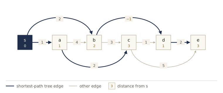
D laid out in topological order, so every edge points right. Processing the vertices left to right, each one's distance is final before its outgoing edges are updated. Navy edges form the shortest-path tree; one edge has negative length.Correctness is the argument we just gave: when we reach \(u\) in the order, every edge into \(u\) comes from an earlier vertex and has already been updated, so \(\text{dist}(u)\) is final (formally, induction along the topological order). The running time is \(O(\lvert V \rvert + \lvert E \rvert)\): linear for the DFS, and then each edge is updated once.
Longest paths
Nothing in the DAG algorithm cares about the sign of the lengths, and that has a useful consequence. The longest path problem — find the path of greatest total length — is hard in general graphs (we will see in module 07 that it is NP-complete), but in a DAG it is easy: negate every length, find shortest paths, and negate the answers. A longest path in the original graph is a shortest path in the negated one, and a DAG has no cycles to go negative around.
Longest paths in DAGs have a classic application: if the vertices are tasks and an edge \((u, v)\) of length \(\ell\) means “\(v\) can start \(\ell\) days after \(u\) starts”, the longest path from the first task gives the earliest possible start of every other task, and the longest path overall, the critical path, determines how long the whole project takes.
def dag_longest_paths(G, s):
    """Longest paths from s in a DAG: shortest paths with every length negated."""
    negated = {u: [(v, -w) for v, w in G[u]] for u in G}
    dist, prev = dag_shortest_paths(negated, s)
    return {u: -d for u, d in dist.items()}, prev

longest, prev = dag_longest_paths(D, "s")
print(longest)
print("longest path to e:", " -> ".join(path_to(prev, "e")), "  length", longest["e"])
{'e': 13, 'd': 9, 'c': 8, 'b': 5, 'a': 1, 's': 0}
longest path to e: s -> a -> b -> c -> e   length 13
Checking the algorithms against each other
We now have many ways to compute shortest paths, with different requirements. Where their domains overlap they must agree, and for small graphs they must all agree with brute force. The brute force from the BFS section extends to lengths directly.
def brute_force_dist(G, s):
    """Shortest distances by trying every simple path from s.
    Exponential time; valid when there is no negative cycle."""
    best = {u: INF for u in G}
    def extend(u, length, on_path):
        best[u] = min(best[u], length)
        for v, w in G[u]:
            if v not in on_path:
                on_path.add(v)
                extend(v, length + w, on_path)
                on_path.remove(v)
    extend(s, 0, {s})
    return best

def unit(G):
    """Give every edge of an unweighted graph length 1."""
    return {u: [(v, 1) for v in G[u]] for u in G}

def random_dag(n, m, rng, lo, hi):
    """A random DAG on 0..n-1. Edges go forward in a hidden random order,
    so 0, 1, ..., n-1 is usually not a topological order."""
    order = list(range(n))
    rng.shuffle(order)
    pairs = [(order[i], order[j]) for i in range(n) for j in range(i + 1, n)]
    G = {u: [] for u in range(n)}
    for u, v in rng.sample(pairs, min(m, len(pairs))):
        G[u].append((v, rng.randint(lo, hi)))
    return G

rng = random.Random(6)
passed = {"unit lengths": 0, "positive lengths": 0, "DAG, any signs": 0}
for _ in range(300):
    n = rng.randint(1, 7)
    m = rng.randint(0, n * (n - 1))
    # unit lengths: BFS, Dijkstra (both versions), Bellman-Ford, brute force
    U = random_digraph(n, m, rng)
    answers = [bfs(U, 0)[0], dijkstra(unit(U), 0)[0],
               dijkstra_pq(unit(U), 0, BinaryHeap())[0],
               bellman_ford(unit(U), 0)[0], brute_force_dist(unit(U), 0)]
    passed["unit lengths"] += all(a == answers[0] for a in answers)
    # positive integer lengths: also the other queues, splitting, and alarm clocks
    P = random_weighted(n, m, rng, 1, 9)
    answers = [dijkstra(P, 0)[0], dijkstra_pq(P, 0, ArrayPQ())[0],
               dijkstra_pq(P, 0, BinaryHeap())[0], dijkstra_pq(P, 0, DaryHeap(3))[0],
               bellman_ford(P, 0)[0], brute_force_dist(P, 0)]
    split = bfs(subdivide(P), 0)[0]
    answers.append({v: split[v] for v in P})
    alarms = alarm_clock(P, 0)
    answers.append({v: alarms.get(v, INF) for v in P})
    passed["positive lengths"] += all(a == answers[0] for a in answers)
    # DAGs with negative lengths: DAG algorithm, Bellman-Ford, brute force
    A = random_dag(n, m, rng, -9, 9)
    answers = [dag_shortest_paths(A, 0)[0], bellman_ford(A, 0)[0], brute_force_dist(A, 0)]
    passed["DAG, any signs"] += all(a == answers[0] for a in answers)
print(passed, "out of 300 each")
{'unit lengths': 300, 'positive lengths': 300, 'DAG, any signs': 300} out of 300 each
General graphs with negative lengths may contain negative cycles, so the check there has two cases: either Bellman–Ford returns distances, which must match brute force, or it reports a cycle, which must be a real cycle of the graph with negative length.
rng = random.Random(8)
outcome = {"distances match": 0, "negative cycle confirmed": 0, "failed": 0}
for _ in range(2000):
    n = rng.randint(2, 7)
    Gn = random_weighted(n, rng.randint(1, n * (n - 1)), rng, -4, 9)
    try:
        good = bellman_ford(Gn, 0)[0] == brute_force_dist(Gn, 0)
        outcome["distances match" if good else "failed"] += 1
    except NegativeCycleError as err:
        cyc = err.cycle  # path_length checks every step is an edge
        good = cyc[0] == cyc[-1] and path_length(Gn, cyc) < 0
        outcome["negative cycle confirmed" if good else "failed"] += 1
print(outcome)
{'distances match': 1207, 'negative cycle confirmed': 793, 'failed': 0}
Brute force cannot handle large graphs, but there a different check works: a certificate. Suppose dist and prev satisfy (a) \(\text{dist}(s) = 0\), (b) \(\text{dist}(v) \le \text{dist}(u) + \ell(u, v)\) for every edge with \(\text{dist}(u)\) finite, and (c) for every reachable \(v \ne s\), the edge from \(\text{prev}(v)\) is tight, \(\text{dist}(v) = \text{dist}(\text{prev}(v)) + \ell(\text{prev}(v), v)\), and following prev pointers leads back to \(s\). Then (c) exhibits a path of length \(\text{dist}(v)\), and (b), summed along any path, shows no path is shorter. So dist is exactly right — and checking (a)–(c) takes linear time.
def certify(G, s, dist, prev):
    """Do dist and prev satisfy the certificate conditions (a)-(c)?"""
    if dist[s] != 0:
        return False
    for u in G:
        for v, w in G[u]:
            if dist[u] + w < dist[v]:  # (b) fails
                return False
    for v in G:
        if v != s and dist[v] < INF:
            u = prev[v]
            if u is None or dist[u] + dict(G[u])[v] != dist[v]:
                return False  # (c) fails: not tight
            if path_to(prev, v)[0] != s:
                return False  # (c) fails: no path to s
    return True

rng = random.Random(7)
results = []
for _ in range(20):
    P = random_weighted(300, 3000, rng, 1, 50)
    d1, p1 = dijkstra(P, 0)
    d2, p2 = dijkstra_pq(P, 0, BinaryHeap())
    d3, p3 = bellman_ford(P, 0)
    A = random_dag(300, 3000, rng, -50, 50)
    d4, p4 = dag_shortest_paths(A, 0)
    d5, p5 = bellman_ford(A, 0)
    results.append(d1 == d2 == d3 and d4 == d5
                   and certify(P, 0, d1, p1) and certify(P, 0, d3, p3)
                   and certify(A, 0, d4, p4) and certify(A, 0, d5, p5))
print(sum(results), "of", len(results), "large random graphs: all algorithms agree,",
      "and every tree is certified")
20 of 20 large random graphs: all algorithms agree, and every tree is certified
Summary
| Edge lengths | Algorithm | Running time |
|---|---|---|
| all equal to 1 | breadth-first search | \(O(\lvert V \rvert + \lvert E \rvert)\) |
| non-negative | Dijkstra with a binary heap | \(O((\lvert V \rvert + \lvert E \rvert) \log \lvert V \rvert)\) |
| non-negative, dense graph | Dijkstra with an unordered array | \(O(\lvert V \rvert^2)\) |
| any, no negative cycle (or detect one) | Bellman–Ford | \(O(\lvert V \rvert \cdot \lvert E \rvert)\) |
| any, graph is a DAG | updates in topological order | \(O(\lvert V \rvert + \lvert E \rvert)\) |
Ideas to carry forward:
- A single-source shortest-path computation returns a whole shortest-path tree, stored as prev pointers; any path is read off by walking back from its end.
- Every algorithm in this module is a sequence of safe updates \(\text{dist}(v) \leftarrow \min\{\text{dist}(v), \text{dist}(u) + \ell(u, v)\}\). They differ only in how they choose the order: layer by layer (BFS), closest vertex first (Dijkstra), everything repeatedly (Bellman–Ford), or topological order (DAGs).
- The running time of an algorithm built on a data structure is a count of operations times their cost. Count the operations first; then choose the structure (array, binary heap, d-ary heap) that makes the most frequent operations cheap for your inputs.
Exercises
- Run
bfson the nine-vertex graphGfrom the first section, starting fromh. List the layers and the queue contents after each ejection, and draw the BFS tree. Then prove that in an undirected graph, every edge joins two vertices whose BFS distances from \(s\) differ by at most 1. What is the corresponding statement for a directed graph, and why is it weaker? - Some graphs have edges of length 0 and 1 only. Modify BFS to use a double-ended queue: a vertex reached by a 0-edge is put at the front of the deque, one reached by a 1-edge at the back. Explain why this computes correct distances in \(O(\lvert V \rvert + \lvert E \rvert)\) time, implement it, and test it against
dijkstraon random graphs. - Draw a graph with five vertices and non-negative edge lengths of your choice, and run Dijkstra’s algorithm on it by hand, recording
distafter each delete-min. Then check your table with thetraceoption ofdijkstra. - Where exactly does the correctness proof of Dijkstra’s algorithm use that lengths are non-negative? Show that edges of length 0 cause no problem. Then give a graph with one negative edge on which Dijkstra’s algorithm still returns correct distances, and explain why it does.
- Build, for every \(n\), a graph with \(n\) vertices and \(n(n-1)/2\) edges on which Dijkstra’s algorithm performs a successful update on every edge. (Hint: vertices \(0, \dots, n-1\), edges from \(i\) to every \(j > i\), with lengths chosen so that each newly finished vertex offers a slightly better route to every later vertex.) Confirm with
dijkstra_pqthat the number of inserts plus decrease-keys is \(n(n-1)/2\). - Suppose you only need the distance from \(s\) to one target \(t\). Modify
dijkstrato stop as soon as \(t\) is finished and prove the result correct. Measure how many vertices are finished on a \(50 \times 50\) grid graph with unit lengths when \(s\) is the center and \(t\) is a neighbor of \(s\). - In a 1-indexed d-ary heap, show that the children of node \(j\) are \((j-1)d + 2, \dots, (j-1)d + d + 1\) and its parent is \(\lfloor (j-2)/d \rfloor + 1\). Then show that choosing \(d = \max(2, \lceil \lvert E \rvert / \lvert V \rvert \rceil)\) gives Dijkstra’s algorithm a running time of \(O(\lvert V \rvert^2)\) on graphs with \(\lvert E \rvert = \Theta(\lvert V \rvert^2)\) and \(O(\lvert V \rvert \log \lvert V \rvert)\) on graphs with \(\lvert E \rvert = O(\lvert V \rvert)\).
- Prove that when round \(\lvert V \rvert\) of Bellman–Ford improves some
distvalue, following prev pointers backward from the improved vertex eventually repeats a vertex, and that the cycle found this way has negative total length. (Hint: along any cycle of prev pointers, add up the inequalities \(\text{dist}(v) \ge \text{dist}(\text{prev}(v)) + \ell(\text{prev}(v), v)\) and look at the edge that was updated last.) - Modify
bellman_fordso that instead of raising an exception it returns, for each vertex, its true distance, which may be \(-\infty\) for vertices reachable from a negative cycle. Your algorithm should still run in \(O(\lvert V \rvert \cdot \lvert E \rvert)\) time. - Suppose the edges of a DAG are given to Bellman–Ford in an order in which each edge \((u, v)\) comes after every edge into \(u\). How many rounds does the algorithm need (including the round that detects that nothing changes)? Compare with
dag_shortest_paths. - Each link of a communication network works with some probability \(p_e \in (0, 1]\), independently of the others, and a message follows a single path. Show how to find the path most likely to deliver a message from \(s\) to \(t\) with one run of Dijkstra’s algorithm, using lengths \(-\log p_e\). Why are these lengths non-negative? Implement it on a small example.
- In your own words: explain to a classmate why Dijkstra’s algorithm needs non-negative lengths, why the DAG algorithm does not, and what Bellman–Ford pays for not needing either assumption.
Going further
- Dasgupta, Papadimitriou, and Vazirani, Algorithms, chapter 4 — the source for this module. Exercises 4.1–4.2 practice the algorithms by hand; 4.8, 4.9, and 4.17 probe the limits of Dijkstra’s algorithm; 4.16 works through the heap implementation; 4.21 applies negative cycles to currency exchange.
- Edsger W. Dijkstra, “A note on two problems in connexion with graphs”, Numerische Mathematik 1 (1959) — the original three-page paper, which also contains an algorithm for minimum spanning trees.
- Michael L. Fredman and Robert E. Tarjan, “Fibonacci heaps and their uses in improved network optimization algorithms”, Journal of the ACM 34 (1987) — the paper behind the last row of the priority-queue table.
- Python documentation:
heapq, whose “Priority Queue Implementation Notes” discuss the lazy-deletion technique used indijkstra. - Robert E. Tarjan, Data Structures and Network Algorithms (SIAM, 1983) — a compact treatment of heaps and shortest-path algorithms, including the d-ary heap analysis.
These notes follow the chapters of S. Dasgupta, C. H. Papadimitriou, and U. V. Vazirani, Algorithms (McGraw-Hill, 2008), the course text. The explanations, code, figures, and exercises here are written for this course; the book remains the reference, with many more exercises.