CSE 431/531 · Module 06 · Week 5
Dynamic Programming
Subproblems and DAGs, longest increasing subsequences, edit distance, knapsack, chain matrix multiplication, and all-pairs shortest paths.
Companion reading: Dasgupta, Papadimitriou & Vazirani, Algorithms, chapter 6, “Dynamic programming”
By the end of this module you can
- Design a dynamic program in three steps — subproblems, a recurrence, an order — and read its running time off the DAG of subproblems.
- Find a longest increasing subsequence in \(O(n^2)\) time, recover it with back pointers, and explain why the same recurrence run as plain recursion takes exponential time.
- Compute the edit distance of two strings by filling an \((m+1) \times (n+1)\) table, recover an optimal alignment, and describe the table as a shortest-path problem on a grid DAG.
- Solve knapsack with and without repetition in \(O(nW)\) time, and explain why that bound is not polynomial in the input size.
- Find the cheapest order for a chain of matrix products in \(O(n^3)\) time using subproblems on intervals.
- Adapt the DP view to shortest paths with at most \(k\) edges, all-pairs shortest paths (Floyd–Warshall), and the traveling salesman problem in \(O(n^2 2^n)\) time.
- Find a largest independent set in a tree in linear time with subproblems on rooted subtrees.
- Choose between bottom-up tables and top-down memoization for a given recurrence.
Contents
- Shortest paths in DAGs, revisited
- Longest increasing subsequences
- Edit distance
- Knapsack
- Chain matrix multiplication
- Shortest paths
- Independent sets in trees
- Summary
- Exercises
- Going further
The design strategies so far each fit a particular shape of problem. Divide and conquer needs a problem that splits into a few much smaller, independent pieces. Graph search needs a graph. The greedy method of module 05 needs a problem where a locally best choice can never hurt, and we saw that most problems do not have that property. This module introduces a technique with a much wider reach: dynamic programming. It solves a problem by identifying a collection of smaller subproblems, solving them from the smallest up, and storing every answer so that nothing is ever computed twice.
You have already met the idea twice. In module 00, fib2 computed Fibonacci numbers by filling a table from \(F_0\) upward, and fib_memo got the same effect by caching a recursive function. In module 04, shortest paths in a DAG took one pass over the nodes in topological order. We start from that second example, because it contains the whole method in miniature: every dynamic program is, underneath, a computation over a DAG whose nodes are subproblems.
Then we apply the method to a series of problems, each teaching one new way of choosing subproblems: longest increasing subsequences (prefixes of one sequence), edit distance (prefixes of two strings), knapsack (smaller capacities, fewer items), chain matrix multiplication (intervals), three shortest-path problems (extra parameters and subsets), and independent sets in trees (subtrees). Along the way we check every algorithm against brute force.
Shortest paths in DAGs, revisited
Recall the key property of a directed acyclic graph (DAG): its nodes can be linearized, or topologically ordered, so that every edge goes from an earlier node to a later one. Take the DAG below, where each node maps to its list of (successor, length) pairs, the weighted representation from module 04.
import math

dag = {
    "s": [("a", 2), ("b", 5)],
    "a": [("b", 1), ("c", 6), ("d", 3)],
    "b": [("d", 1)],
    "c": [("t", 1)],
    "d": [("c", 1), ("t", 4)],
    "t": [],
}

def topological_order(graph):
    """Nodes ordered so that every edge goes left to right (reverse DFS post-order)."""
    seen, post = set(), []
    def explore(u):
        seen.add(u)
        for v, _ in graph[u]:
            if v not in seen:
                explore(v)
        post.append(u)
    for u in graph:
        if u not in seen:
            explore(u)
    return post[::-1]

def predecessors(graph):
    """The reverse graph: for each node v, the (u, length) pairs with an edge u -> v."""
    pred = {v: [] for v in graph}
    for u in graph:
        for v, w in graph[u]:
            pred[v].append((u, w))
    return pred

topological_order(dag)
['s', 'a', 'b', 'd', 'c', 't']
Suppose we want the distance from s to t. Every path into t arrives along one of its incoming edges, from c (length 1) or from d (length 4), so
The same holds at every node \(v\): \(\text{dist}(v)\) is the minimum, over the edges \((u, v)\) into \(v\), of \(\text{dist}(u) + \ell(u, v)\). If we visit the nodes in topological order, the distances on the right-hand side are always known by the time we need them, so one pass computes everything.
def dag_distances(graph, s, best=min):
    """dist(v) from s for every node, one node at a time in topological order.
    With best=max it computes longest-path lengths instead."""
    pred = predecessors(graph)
    unreached = math.inf if best is min else -math.inf
    dist = {}
    for v in topological_order(graph):
        if v == s:
            dist[v] = 0
        else:
            dist[v] = best((dist[u] + w for u, w in pred[v]), default=unreached)
    return dist

print("shortest:", dag_distances(dag, "s"))
print("longest: ", dag_distances(dag, "s", best=max))
shortest: {'s': 0, 'a': 2, 'b': 3, 'd': 4, 'c': 5, 't': 6}
longest:  {'s': 0, 'a': 2, 'b': 5, 'd': 6, 'c': 8, 't': 10}
The shortest path to t has length 6 (it is s a b d c t); the longest has length 10 (s b d t). Changing one word, min to max, turned one problem into another. Longest paths are hard in general graphs, as we will see in module 07, but in a DAG they are as easy as shortest ones. Replacing the sum by a product would give paths with the smallest product of edge lengths, and so on: the method only needs some rule that combines the values at a node’s predecessors.
Subproblems form a DAG
Look at what the algorithm did. It solved a collection of subproblems, the values \(\{\text{dist}(v) : v \in V\}\). It started with the smallest one, \(\text{dist}(s) = 0\), and worked toward “larger” ones, where a subproblem counts as larger if it needs the answers to more subproblems before it can be solved. That is the whole of dynamic programming.
Definition. A dynamic program consists of (1) a collection of subproblems, (2) a recurrence that expresses the answer to each subproblem in terms of answers to smaller subproblems, and (3) an order in which every subproblem comes after all the subproblems it depends on. Draw an edge \(A \to B\) whenever solving \(B\) uses the answer to \(A\): the result is the subproblem DAG, and a valid order is a topological order of it.
In the shortest-path example, the subproblem DAG is the input graph itself. From now on it will not be: we will invent the subproblems, and the DAG is implicit in the recurrence. For fib2, the subproblems are \(F_0, \dots, F_n\) and each \(F_i\) has edges from \(F_{i-1}\) and \(F_{i-2}\). The difficult, creative step is always the first one: choosing subproblems that are few in number and that satisfy a recurrence. Once that is done, the algorithm writes itself.
Longest increasing subsequences
The problem
Given a sequence of numbers \(a_1, \dots, a_n\), a subsequence is any selection of its elements kept in their original order: \(a_{i_1}, a_{i_2}, \dots, a_{i_k}\) with \(i_1 < i_2 < \dots < i_k\). The selected elements need not be adjacent. A subsequence is increasing if each element is strictly larger than the one before. The longest increasing subsequence problem asks for an increasing subsequence of maximum length.
Take the sequence 3, 8, 1, 6, 4, 9, 5, 7. The subsequence 3, 6, 9 is increasing, of length 3. The subsequence 3, 4, 5, 7 is longer, and you can check that no increasing subsequence has length 5. There can be several optimal answers: 1, 4, 5, 7 also has length 4.
A brute-force algorithm would try all \(2^n\) subsequences. We can do much better once we see the right picture.
A DAG hiding in the sequence
Make one node for each position \(j\), and draw an edge \(i \to j\) whenever \(a_i\) and \(a_j\) could be consecutive elements of an increasing subsequence, that is, whenever \(i < j\) and \(a_i < a_j\).
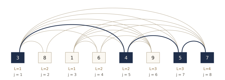
Two facts make this graph useful. It is a DAG, because every edge goes from a smaller index to a larger one (so the positions \(1, \dots, n\) are already a topological order). And increasing subsequences correspond one-to-one to paths in it. So the problem is: find a longest path in a DAG, which we just saw how to do.
The recurrence
Let \(L(j)\) be the length of the longest increasing subsequence that ends at position \(j\) (the number of nodes on the longest path ending at \(j\)). Such a subsequence is either \(a_j\) alone, or a longest increasing subsequence ending at some predecessor \(i\) of \(j\), extended by \(a_j\):
\[L(j) = 1 + \max\{L(i) : i < j \text{ and } a_i < a_j\},\]where the maximum of an empty set is 0. The answer is \(\max_j L(j)\), since the subsequence may end anywhere. To recover the subsequence, not only its length, record for each \(j\) the predecessor \(\text{prev}(j)\) that achieved the maximum — the same back-pointer device used for shortest paths in module 04 — and follow the pointers back from the best end.
In Python, positions are numbered from 0 rather than 1; otherwise the code is the recurrence.
def lis(a):
    """Return (L, s): L[j] = length of the longest increasing subsequence ending at a[j],
    and s = one longest increasing subsequence of a."""
    n = len(a)
    L = [1] * n
    prev = [None] * n
    for j in range(n):
        for i in range(j):
            if a[i] < a[j] and L[i] + 1 > L[j]:
                L[j], prev[j] = L[i] + 1, i
    if n == 0:
        return L, []
    j = max(range(n), key=lambda k: L[k])       # where a longest one ends
    s = []
    while j is not None:                        # follow the back pointers
        s.append(a[j])
        j = prev[j]
    return L, s[::-1]

L, s = lis([3, 8, 1, 6, 4, 9, 5, 7])
print("L =", L)
print("longest increasing subsequence:", s)
L = [1, 2, 1, 2, 2, 3, 3, 4]
longest increasing subsequence: [3, 4, 5, 7]
The table L matches the values in the figure. The back pointers lead from 7 to 5 to 4 to 3.
Correctness and running time
Correctness. By induction on \(j\). An increasing subsequence ending at \(a_j\) is either \(a_j\) alone or has a next-to-last element \(a_i\) with \(i < j\) and \(a_i < a_j\); removing \(a_j\) leaves an increasing subsequence ending at \(a_i\), of length at most \(L(i)\) by induction. So no increasing subsequence ending at \(a_j\) is longer than the right-hand side. Conversely, appending \(a_j\) to a longest one ending at the best \(i\) achieves it. Because the loop visits \(j\) in increasing order, every \(L(i)\) it reads has already been computed.
Running time. The work for \(L(j)\) is proportional to the number of candidates \(i < j\), so the total is \(1 + 2 + \dots + (n - 1) = O(n^2)\). Put in terms of the DAG: the work is proportional to the number of nodes plus the number of edges, and a DAG on \(n\) positions has at most \(n(n-1)/2\) edges (all of them present when the input is sorted). This is the first instance of a rule we will use repeatedly: the running time of a dynamic program is about the number of edges in its subproblem DAG.
An \(O(n \log n)\) algorithm for this problem also exists (exercise 2), but the quadratic one is the model for everything that follows.
Checking against brute force
For short sequences we can try every subsequence, longest first, and compare. Random sequences with repeated values also test that we insist on strictly increasing.
import random
from itertools import combinations

def lis_brute(a):
    """Length of a longest increasing subsequence: try all index sets, longest first."""
    for k in range(len(a), 0, -1):
        for idx in combinations(range(len(a)), k):
            if all(a[p] < a[q] for p, q in zip(idx, idx[1:])):
                return k
    return 0

def is_increasing_subsequence(s, a):
    """Is s strictly increasing and a subsequence of a?"""
    it = iter(a)
    return all(x < y for x, y in zip(s, s[1:])) and all(x in it for x in s)

random.seed(1)
trials = 0
for _ in range(500):
    a = [random.randint(0, 9) for _ in range(random.randint(0, 10))]
    L, s = lis(a)
    assert len(s) == lis_brute(a) and is_increasing_subsequence(s, a)
    trials += 1
print(f"{trials} random sequences: lis agrees with brute force")
500 random sequences: lis agrees with brute force
The helper is_increasing_subsequence uses a small Python idiom: x in it advances the iterator it past the first match, so the second all checks that the elements of s appear in a in order.
Recursion without memory is exponential
The recurrence for \(L(j)\) suggests an even shorter program: a recursive function that calls itself on every valid \(i < j\). It is correct, but it is a very bad idea. Let us count its calls on a sorted input, where every \(i < j\) is a valid predecessor.
def naive_calls(a, j):
    """Number of calls made by L(j) computed by plain recursion on the recurrence."""
    calls = 0
    def L(j):
        nonlocal calls
        calls += 1
        return 1 + max((L(i) for i in range(j) if a[i] < a[j]), default=0)
    L(j)
    return calls

for n in [5, 10, 15, 20]:
    calls = naive_calls(list(range(n)), n - 1)
    print(f"n = {n:2d}: calls for L(n) = {calls:>7,}   2^(n-1) = {2 ** (n - 1):>7,}")
n =  5: calls for L(n) =      16   2^(n-1) =      16
n = 10: calls for L(n) =     512   2^(n-1) =     512
n = 15: calls for L(n) =  16,384   2^(n-1) =  16,384
n = 20: calls for L(n) = 524,288   2^(n-1) = 524,288
Exactly \(2^{n-1}\). If \(T(j)\) is the number of calls made by \(L(j)\), then \(T(1) = 1\) and \(T(j) = 1 + T(1) + \dots + T(j-1)\), so each \(T(j)\) is twice the previous one. Yet there are only \(n\) distinct subproblems; the recursion solves each of them an exponential number of times, just like fib1 in module 00.
Why did recursion serve us so well in divide and conquer, and fail here? In mergesort, a problem of size \(n\) calls subproblems of size \(n/2\). The sizes drop so fast that the recursion tree has logarithmic depth and a polynomial number of nodes, and the subproblems are disjoint. In a typical dynamic program, a subproblem depends on others that are only slightly smaller (\(L(j)\) uses \(L(j-1)\)), so the recursion tree has linear depth and exponentially many nodes. The saving grace is that almost all of those nodes are repeats: there are few distinct subproblems. Efficiency comes from enumerating them and solving each once.
Watch out. A correct recurrence is not yet an efficient algorithm. Run directly as recursion, it re-solves shared subproblems and usually takes exponential time. Always either fill a table in a valid order or cache the recursive calls.
Memoization: the same recurrence, top-down
There are two ways to make sure each subproblem is solved once. The bottom-up way, used by lis, lists the subproblems in an order that respects the dependencies and fills a table. The top-down way keeps the recursive function but caches its results; as in module 00, this is memoization, and functools.cache does it for us.
from functools import cache

def lis_length_topdown(a):
    """Length of a longest increasing subsequence: the recurrence with a cache."""
    @cache
    def L(j):
        return 1 + max((L(i) for i in range(j) if a[i] < a[j]), default=0)
    return max((L(j) for j in range(len(a))), default=0)

random.seed(2)
tests = [[random.randint(0, 20) for _ in range(random.randint(0, 30))] for _ in range(300)]
print(all(lis_length_topdown(a) == len(lis(a)[1]) for a in tests))
print(lis_length_topdown(list(range(500))))
True
500
The cached version finds the length 500 for a sorted input of length 500 instantly, where the uncached recursion would make \(2^{499}\) calls. Both versions do the same \(O(n^2)\) work. How do they compare?
- Bottom-up needs you to find a valid order, and it solves every subproblem, needed or not. It has no recursion overhead and no limit on depth.
- Top-down finds the order for you: the recursion is a depth-first search of the subproblem DAG, and a subproblem finishes only after everything it depends on has finished. It solves only the subproblems reachable from the one you ask for. But each call costs more than a loop iteration, and deep recursion can hit Python’s recursion limit (about 1,000 frames by default).
We return to this trade-off with knapsack, where the “only what is needed” advantage can be large.
Note. The name has little to do with programming in our sense. Richard Bellman introduced “dynamic programming” in the 1950s, when “programming” meant planning, as in scheduling or logistics, and the method was designed to plan multistage processes optimally. A DAG such as the one above can be read that way: nodes are states of a process, and edges are the decisions that move it from one state to the next.
Edit distance
Alignments and their cost
How close are two strings? A spell checker faced with an unknown word wants the dictionary words that are nearest to it, and it needs a measure of nearness. A natural one comes from alignments. An alignment of strings \(x\) and \(y\) writes one above the other, with gaps (shown as -) inserted anywhere in either string, so that the two rows have the same length and no column holds two gaps. The cost of an alignment is the number of columns in which the two rows differ. The edit distance between \(x\) and \(y\) is the minimum cost over all their alignments.
Here are two alignments of GRAPE and GROUPS, of cost 3 and 4:
\[\begin{array}{cccccc} \texttt{G} & \texttt{R} & \texttt{-} & \texttt{A} & \texttt{P} & \texttt{E} \\ \texttt{G} & \texttt{R} & \texttt{O} & \texttt{U} & \texttt{P} & \texttt{S} \end{array} \qquad\qquad \begin{array}{cccccc} \texttt{G} & \texttt{R} & \texttt{A} & \texttt{P} & \texttt{E} & \texttt{-} \\ \texttt{G} & \texttt{R} & \texttt{O} & \texttt{U} & \texttt{P} & \texttt{S} \end{array}\]The name comes from a second reading. Each column of an alignment is an edit turning \(x\) into \(y\): a column with a gap on top inserts a letter of \(y\), a gap on the bottom deletes a letter of \(x\), and two different letters substitute one for the other. The left alignment says: insert O, substitute A by U, substitute E by S. So the edit distance is also the minimum number of insertions, deletions, and substitutions that turn \(x\) into \(y\). For these two words it is 3, as we will confirm.
Searching all alignments is hopeless. An alignment is a sequence of columns of three kinds — two letters, a letter over a gap, a gap over a letter — so alignments correspond to walks from \((0, 0)\) to \((m, n)\) with steps \((1, 1)\), \((1, 0)\), and \((0, 1)\). Counting them is itself a small dynamic program:
def count_alignments(m, n):
    """Number of alignments of a string of length m with one of length n."""
    N = [[1] * (n + 1) for _ in range(m + 1)]
    for i in range(1, m + 1):
        for j in range(1, n + 1):
            N[i][j] = N[i - 1][j] + N[i][j - 1] + N[i - 1][j - 1]
    return N[m][n]

for n in [5, 10, 20, 40]:
    print(f"two strings of length {n:2d}: {count_alignments(n, n):,} alignments")
two strings of length  5: 1,683 alignments
two strings of length 10: 8,097,453 alignments
two strings of length 20: 260,543,813,797,441 alignments
two strings of length 40: 378,150,244,155,138,145,169,182,750,209 alignments
Subproblems on prefixes
We want the edit distance between \(x[1..m]\) and \(y[1..n]\). What smaller problems would help? A natural guess: the same problem on prefixes. Define
\[E(i, j) = \text{edit distance between } x[1..i] \text{ and } y[1..j], \qquad 0 \le i \le m,\ 0 \le j \le n.\]The answer is \(E(m, n)\). To express \(E(i, j)\) through smaller subproblems, look at the last column of an optimal alignment of \(x[1..i]\) with \(y[1..j]\). It can only be one of three things:
- \(x[i]\) over a gap. This column costs 1, and the columns before it must be an optimal alignment of \(x[1..i-1]\) with \(y[1..j]\): cost \(1 + E(i-1, j)\).
- A gap over \(y[j]\). Cost \(1 + E(i, j-1)\) by the same reasoning.
- \(x[i]\) over \(y[j]\). This column costs 0 if the letters are equal and 1 otherwise; the rest is an alignment of \(x[1..i-1]\) with \(y[1..j-1]\).
We do not know which case holds, so we take the best:
\[E(i, j) = \min\bigl\{ 1 + E(i-1, j),\ \ 1 + E(i, j-1),\ \ \text{diff}(i, j) + E(i-1, j-1) \bigr\},\]where \(\text{diff}(i, j)\) is 0 if \(x[i] = y[j]\) and 1 otherwise. For example, with \(x\) = GRAPE and \(y\) = GROUPS, the subproblem \(E(3, 4)\) compares GRA with GROU. The last column of its best alignment is A over a gap, a gap over U, or A over U, so \(E(3, 4) = \min\{1 + E(2, 4),\ 1 + E(3, 3),\ 1 + E(2, 3)\}\).
The smallest subproblems are those with an empty prefix. Aligning \(j\) letters with the empty string needs \(j\) columns of the form gap-over-letter, so \(E(0, j) = j\), and likewise \(E(i, 0) = i\).
Why is the “rest must be optimal” step valid? If the columns before the last one were not an optimal alignment of the remaining prefixes, we could replace them with a cheaper one and lower the total, contradicting optimality. This cut-and-paste argument, that an optimal solution is built from optimal solutions to subproblems, is the heart of every correctness proof in this module.
Filling the table
The answers \(E(i, j)\) form a two-dimensional table. Entry \((i, j)\) depends on its neighbors above, to the left, and diagonally above-left, so any order that handles those three before \((i, j)\) is valid. Row by row, left to right, is the simplest.
def edit_distance_table(x, y):
    """E[i][j] = edit distance between x[:i] and y[:j]."""
    m, n = len(x), len(y)
    E = [[0] * (n + 1) for _ in range(m + 1)]
    for i in range(m + 1):
        E[i][0] = i
    for j in range(n + 1):
        E[0][j] = j
    for i in range(1, m + 1):
        for j in range(1, n + 1):
            diff = 0 if x[i - 1] == y[j - 1] else 1
            E[i][j] = min(E[i - 1][j] + 1,          # x[i] over a gap
                          E[i][j - 1] + 1,          # a gap over y[j]
                          E[i - 1][j - 1] + diff)   # x[i] over y[j]
    return E

def show_table(x, y, E):
    """Print the table with y across the top and x down the side."""
    print("      " + "".join(c.rjust(3) for c in y))
    for i, row in enumerate(E):
        label = x[i - 1] if i > 0 else " "
        print(label.rjust(3) + "".join(str(v).rjust(3) for v in row))

E = edit_distance_table("GRAPE", "GROUPS")
show_table("GRAPE", "GROUPS", E)
        G  R  O  U  P  S
     0  1  2  3  4  5  6
  G  1  0  1  2  3  4  5
  R  2  1  0  1  2  3  4
  A  3  2  1  1  2  3  4
  P  4  3  2  2  2  2  3
  E  5  4  3  3  3  3  3
The bottom-right entry, \(E(5, 6) = 3\), is the edit distance between GRAPE and GROUPS, so the left-hand alignment above is optimal. Other entries answer smaller questions: row P, column U says that GRAP and GROU are at distance 2, and the zeros along the diagonal at the top left record the common prefix GR.
Recovering the alignment
The table stores only costs. To recover an optimal alignment, start at \((m, n)\) and ask which of the three cases produced the entry; step to that neighbor, emit the corresponding column, and repeat until \((0, 0)\). We prefer the diagonal when several cases tie.
def alignment(x, y, E):
    """One optimal alignment, traced back through the table from (m, n) to (0, 0)."""
    top, bottom = [], []
    i, j = len(x), len(y)
    while i > 0 or j > 0:
        if i > 0 and j > 0 and E[i][j] == E[i - 1][j - 1] + (x[i - 1] != y[j - 1]):
            top.append(x[i - 1]); bottom.append(y[j - 1]); i, j = i - 1, j - 1
        elif i > 0 and E[i][j] == E[i - 1][j] + 1:
            top.append(x[i - 1]); bottom.append("-"); i -= 1
        else:
            top.append("-"); bottom.append(y[j - 1]); j -= 1
    return "".join(reversed(top)), "".join(reversed(bottom))

def edit_distance(x, y):
    E = edit_distance_table(x, y)
    return E[len(x)][len(y)], alignment(x, y, E)

d, (top, bottom) = edit_distance("GRAPE", "GROUPS")
print("edit distance", d)
print(top)
print(bottom)
edit distance 3
GR-APE
GROUPS
The traceback reproduces the left-hand alignment from the start of the section: match G and R, insert O, substitute A by U, match P, substitute E by S.
Correctness, running time, and a check
Correctness follows from the case analysis above, by induction over the table in fill order: the base cases are right, and each entry is the minimum over the only three possible last columns, each combined with an optimal (by induction) alignment of the remaining prefixes. The table has \((m+1)(n+1)\) entries and each takes constant time, so the running time is \(O(mn)\), and so is the memory.
As a check, here is the recurrence run as plain recursion, with no table. It considers every alignment implicitly, so it is a brute-force answer; it is exponential, which is fine for strings of length at most 6. We also confirm that each traced alignment has the claimed cost and really spells out \(x\) and \(y\) once the gaps are removed.
def edit_distance_brute(x, y):
    """The recurrence as plain recursion: exponential time, fine for tiny strings."""
    if not x:
        return len(y)
    if not y:
        return len(x)
    return min(1 + edit_distance_brute(x[:-1], y),
               1 + edit_distance_brute(x, y[:-1]),
               (x[-1] != y[-1]) + edit_distance_brute(x[:-1], y[:-1]))

random.seed(3)
for _ in range(300):
    x = "".join(random.choice("abc") for _ in range(random.randint(0, 6)))
    y = "".join(random.choice("abc") for _ in range(random.randint(0, 6)))
    d, (top, bottom) = edit_distance(x, y)
    assert d == edit_distance_brute(x, y)
    assert top.replace("-", "") == x and bottom.replace("-", "") == y
    assert d == sum(p != q for p, q in zip(top, bottom))
print("300 random pairs: table, traceback, and brute force agree")
300 random pairs: table, traceback, and brute force agree
The underlying DAG
Every dynamic program has a subproblem DAG, and for edit distance it is a grid. There is a node for each table position \((i, j)\) and an edge into \((i, j)\) from each of the three positions it depends on: \((i-1, j)\), \((i, j-1)\), and \((i-1, j-1)\). We can go one step further and put lengths on the edges: length 1 on every edge, except length 0 on a diagonal edge into \((i, j)\) when \(x[i] = y[j]\). Then the recurrence for \(E(i, j)\) is exactly the shortest-path recurrence from the first section, and the edit distance is the length of a shortest path from \((0, 0)\) to \((m, n)\).
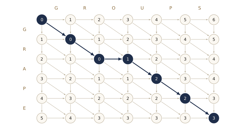
On the highlighted path, the three zero-length diagonals are the matches G, R, and P, and the three unit-length steps are the insertion of O and the two substitutions. Changing the edge lengths gives variants of edit distance for free: if substitutions should cost 2, or deleting a vowel should be cheap, put those numbers on the corresponding edges and run the same algorithm.
Note. Alignment is a basic tool in computational biology. DNA is a long string over the alphabet A, C, G, T, and one way to guess the role of a newly sequenced gene is to find known genes that align with it at low cost. Biologists use weighted variants of edit distance, with scores for each pair of letters and for gaps, and the dynamic program is the same grid computation with different edge lengths (DPV exercises 6.26–6.28 develop this).
Time and memory from the DAG
Two rules of thumb follow from the DAG view.
- Time. A dynamic program visits the nodes of its subproblem DAG in topological order and, for each node, looks at its incoming edges, usually doing constant work per edge. So the running time is proportional to the number of nodes plus edges. For edit distance that is \(O(mn)\) nodes and three edges per node.
- Memory. A subproblem’s answer must be kept only until every subproblem that depends on it has been solved. The edit-distance table is filled row by row and each row depends only on the row above, so two rows suffice. Swapping the strings so that the rows run along the shorter one, memory drops to \(O(\min(m, n))\).
def edit_distance_two_rows(x, y):
    """Edit distance keeping two rows of the table, each as long as the shorter string."""
    if len(y) > len(x):
        x, y = y, x                     # edit distance is symmetric
    prev = list(range(len(y) + 1))      # row 0
    for i in range(1, len(x) + 1):
        cur = [i] + [0] * len(y)
        for j in range(1, len(y) + 1):
            cur[j] = min(prev[j] + 1, cur[j - 1] + 1,
                         prev[j - 1] + (x[i - 1] != y[j - 1]))
        prev = cur
    return prev[-1]

random.seed(4)
pairs = [("".join(random.choices("acgt", k=random.randint(0, 40))),
          "".join(random.choices("acgt", k=random.randint(0, 40)))) for _ in range(200)]
print(all(edit_distance_two_rows(x, y) == edit_distance(x, y)[0] for x, y in pairs))
True
The saving comes at a price: with only two rows we can no longer trace back the alignment. (There is a clever divide-and-conquer method that recovers the alignment in linear space too; see Going further.)
Choosing subproblems
Finding the right subproblems takes practice, but a few patterns cover most of what you will meet. We have now seen the first two; the other two are coming.
| Input | Subproblem | Number of subproblems | Example in this module |
|---|---|---|---|
| a sequence \(x_1, \dots, x_n\) | a prefix \(x_1, \dots, x_i\) | \(n\) | longest increasing subsequence |
| two sequences \(x_1, \dots, x_m\) and \(y_1, \dots, y_n\) | a pair of prefixes \(x_1, \dots, x_i\) and \(y_1, \dots, y_j\) | \(mn\) | edit distance |
| a sequence \(x_1, \dots, x_n\) | a contiguous piece \(x_i, \dots, x_j\) | \(O(n^2)\) | chain matrix multiplication |
| a rooted tree | a subtree hanging from a node | one per node | independent sets in trees |
When none of these fits, the question to ask is the one we will ask for knapsack and the traveling salesman: what do I need to remember about a partial solution in order to extend it? That information becomes the parameters of the subproblem.
Knapsack
The problem
A knapsack can carry a total weight of at most \(W\). There are \(n\) kinds of items; item \(i\) has integer weight \(w_i\) and value \(v_i\). Which items should we pack to maximize the total value? The story is a thief with a bag, but the same problem appears whenever a limited resource — CPU time, bandwidth, a budget — must be spent on tasks with different costs and payoffs.
There are two versions. In knapsack with repetition there is an unlimited supply of each item, so an item can be packed several times. In knapsack without repetition (also called 0–1 knapsack) there is one of each. Our running example has \(W = 11\) and these four items:
| Item | Weight | Value | Value per unit weight |
|---|---|---|---|
| 1 | 8 | 43 | 5.38 |
| 2 | 5 | 32 | 6.40 |
| 3 | 4 | 25 | 6.25 |
| 4 | 3 | 15 | 5.00 |
The greedy idea from module 05, taking items in order of value per unit weight, is not optimal here. Without repetition it takes item 2, then item 3 (total weight 9), and has no room left: value 57. We will see that 58 is possible. Greedy fails, so we turn to dynamic programming. Neither version of knapsack is known to have a polynomial-time algorithm, and in module 07 we will see why one is unlikely to exist; the algorithms below take \(O(nW)\) time, which is fine when \(W\) is small.
Knapsack with repetition
What are the subproblems? We could shrink the capacity or shrink the set of items. With repetition, shrinking the capacity is enough. Let
\[K(w) = \text{the maximum value achievable with a knapsack of capacity } w.\]If an optimal packing for capacity \(w\) contains item \(i\), then removing one copy of it leaves a packing of capacity \(w - w_i\), and that packing must be optimal for \(w - w_i\) (otherwise swap in a better one and beat the optimum). We do not know which \(i\), so we try them all:
\[K(w) = \max_{i \,:\, w_i \le w} \bigl\{ K(w - w_i) + v_i \bigr\},\]with the maximum of an empty set equal to 0 (nothing fits, value 0). The subproblems \(K(0), K(1), \dots, K(W)\) are ordered by capacity. To recover the packing, remember which item achieved each maximum.
items = [(8, 43), (5, 32), (4, 25), (3, 15)]      # (weight, value) of items 1, 2, 3, 4
weights = [w for w, v in items]
values = [v for w, v in items]

def knapsack_rep(W, weights, values):
    """Knapsack with repetition. Returns the best value and the items packed
    (numbered from 1)."""
    K = [0] * (W + 1)
    last = [None] * (W + 1)          # an item in an optimal knapsack of capacity w
    for w in range(1, W + 1):
        for i, (wi, vi) in enumerate(zip(weights, values)):
            if wi <= w and K[w - wi] + vi > K[w]:
                K[w], last[w] = K[w - wi] + vi, i
    packed, w = [], W
    while last[w] is not None:       # remove one item at a time
        packed.append(last[w] + 1)
        w -= weights[last[w]]
    return K[W], sorted(packed)

print(knapsack_rep(11, weights, values))
(65, [3, 3, 4])
With repetition, the best knapsack of capacity 11 holds two copies of item 3 and one of item 4, worth 65. The algorithm fills a one-dimensional table of \(W + 1\) entries, each in \(O(n)\) time, so it runs in \(O(nW)\) time.
There is, as always, a DAG underneath: its nodes are the capacities \(0, 1, \dots, W\), and each item gives an edge \(w - w_i \to w\) of length \(v_i\). The recurrence says \(K(w)\) is the length of the longest path ending at \(w\) — knapsack with repetition is the longest-path problem on this DAG.
Knapsack without repetition
Now each item may be used at most once, and the subproblems \(K(w)\) stop working. Knowing that \(K(w - w_n)\) is large does not help, because we do not know whether that packing already used item \(n\). The subproblem must carry more information: which items are still available. Add a second parameter:
\[K(w, j) = \text{the maximum value achievable with capacity } w \text{ using only items } 1, \dots, j.\]The answer is \(K(W, n)\). For the recurrence, ask the one question that matters about item \(j\): is it in the optimal packing or not?
\[K(w, j) = \max\bigl\{ K(w - w_j, j - 1) + v_j,\ \ K(w, j - 1) \bigr\},\]where the first option is allowed only when \(w_j \le w\). The base cases are \(K(w, 0) = 0\) (no items) and \(K(0, j) = 0\) (no room). Each subproblem depends only on subproblems with \(j - 1\), so we fill the table one item at a time. To recover the packing, walk back from \((W, n)\): item \(j\) was used exactly when \(K(w, j) \ne K(w, j - 1)\).
def knapsack_01(W, weights, values):
    """Knapsack without repetition. Returns the best value and the items packed
    (numbered from 1)."""
    n = len(weights)
    K = [[0] * (n + 1) for _ in range(W + 1)]         # K[w][j]
    for j in range(1, n + 1):
        wj, vj = weights[j - 1], values[j - 1]
        for w in range(1, W + 1):
            K[w][j] = K[w][j - 1]                     # leave item j out
            if wj <= w and K[w - wj][j - 1] + vj > K[w][j]:
                K[w][j] = K[w - wj][j - 1] + vj       # put item j in
    packed, w = [], W
    for j in range(n, 0, -1):
        if K[w][j] != K[w][j - 1]:                    # item j was used
            packed.append(j)
            w -= weights[j - 1]
    return K[W][n], sorted(packed)

print(knapsack_01(11, weights, values))
(58, [1, 4])
Without repetition the best value is 58, from items 1 and 4 (weight exactly 11) — one more than greedy’s 57. The table now has \((W + 1)(n + 1)\) entries but each takes constant time, so the running time is again \(O(nW)\).
Both functions deserve a check against exhaustive search. Without repetition, try all \(2^n\) subsets; with repetition, try every combination of counts \(c_i \le W / w_i\).
from itertools import product

def knapsack_brute(W, weights, values, repetition):
    """Best value by trying every choice of counts (each 0 or 1 without repetition)."""
    ranges = [range(W // w + 1) if repetition else range(2) for w in weights]
    best = 0
    for counts in product(*ranges):
        if sum(c * w for c, w in zip(counts, weights)) <= W:
            best = max(best, sum(c * v for c, v in zip(counts, values)))
    return best

random.seed(5)
for _ in range(200):
    n, W = random.randint(1, 5), random.randint(0, 15)
    ws = [random.randint(1, 8) for _ in range(n)]
    vs = [random.randint(1, 30) for _ in range(n)]
    for solve, rep in [(knapsack_rep, True), (knapsack_01, False)]:
        best, packed = solve(W, ws, vs)
        assert best == knapsack_brute(W, ws, vs, rep)
        assert sum(ws[i - 1] for i in packed) <= W
        assert sum(vs[i - 1] for i in packed) == best
        assert rep or len(set(packed)) == len(packed)
print("200 random instances: both versions agree with brute force")
200 random instances: both versions agree with brute force
Pseudo-polynomial time
Is \(O(nW)\) a polynomial running time? It looks like one, but it is not polynomial in the size of the input. The capacity \(W\) is written with about \(\log_2 W\) bits, so \(W\) itself is exponential in its own length. Multiply every weight and the capacity by 1,000: the input grows by about 10 bits per number, the answer does not change at all, and the table grows a thousandfold.
for scale in [1, 10, 100, 1000]:
    W = 11 * scale
    best, packed = knapsack_rep(W, [w * scale for w in weights], values)
    print(f"W = {W:>6,}: best value {best}, table entries {W + 1:>6,}, "
          f"work n*W = {len(weights) * W:>6,}")
W =     11: best value 65, table entries     12, work n*W =     44
W =    110: best value 65, table entries    111, work n*W =    440
W =  1,100: best value 65, table entries  1,101, work n*W =  4,400
W = 11,000: best value 65, table entries 11,001, work n*W = 44,000
An algorithm whose running time is polynomial in the numeric values in the input, rather than in their length in bits, is called pseudo-polynomial. It is useful when the numbers are small integers (capacities in the hundreds or thousands), and useless when they are large.
Watch out. Always measure input size in bits, as in module 00. An \(O(nW)\) knapsack algorithm is exponential in the length of \(W\); the same caution applies to any algorithm whose table is indexed by a number from the input, such as the change-making problems in the exercises.
Memoization revisited
The scaled instances expose a waste in the bottom-up table. When all weights and the capacity are multiples of 100, the only capacities that can ever matter are multiples of 100, yet the table fills all \(W + 1\) entries. The top-down version only visits the subproblems it actually reaches. Here it is with an explicit dictionary as the cache, so we can count its entries:
def knapsack_rep_memo(W, weights, values):
    """Knapsack with repetition, top-down with a dictionary of solved subproblems."""
    memo = {}
    def K(w):
        if w not in memo:
            memo[w] = max((K(w - wi) + vi for wi, vi in zip(weights, values) if wi <= w),
                          default=0)
        return memo[w]
    return K(W), len(memo)

W = 1100
best, solved = knapsack_rep_memo(W, [100 * w for w in weights], values)
print(f"best value {best}")
print(f"subproblems solved top-down: {solved}; bottom-up table entries: {W + 1}")
best value 65
subproblems solved top-down: 10; bottom-up table entries: 1101
The top-down version solved 10 subproblems — the multiples of 100 from 0 to 1,100, except 900 and 1,000, which no sequence of removals reaches — where the table has 1,101 entries. Both approaches solve each subproblem at most once, so both run in \(O(nW)\) time in the worst case, and when every subproblem is needed the bottom-up table wins by a constant factor (no function calls, no hashing). But the bottom-up table fills in every entry, whether or not the final answer depends on it, while memoization visits only the subproblems the recursion actually reaches. When the reachable subproblems are a small fraction of the table, as here, memoization can be much faster.
Chain matrix multiplication
The cost of a product
Multiplying a \(p \times q\) matrix by a \(q \times r\) matrix with the usual method takes \(pqr\) multiplications of numbers (each of the \(pr\) entries of the result is a dot product of length \(q\)), and we use that as its cost. Suppose we want the product \(A \times B \times C \times D\) of four matrices with dimensions
\[A: 30 \times 2, \qquad B: 2 \times 6, \qquad C: 6 \times 40, \qquad D: 40 \times 20.\]Matrix multiplication is not commutative, but it is associative: \((A \times B) \times C = A \times (B \times C)\). So we may parenthesize the product any way we like and get the same result — at very different costs. The function below lists every parenthesization of \(A_i \times \dots \times A_j\) with its cost, by trying every choice of the last multiplication.
NAMES = "ABCDEFGHIJKLMNOPQRSTUVWXYZ"

def all_orders(m, i, j):
    """Yield (cost, parenthesization) for every way to compute A_i x ... x A_j,
    where matrix A_k has dimensions m[k-1] x m[k]."""
    if i == j:
        yield 0, NAMES[i - 1]
        return
    for k in range(i, j):                 # the last multiplication splits after A_k
        for c1, s1 in all_orders(m, i, k):
            for c2, s2 in all_orders(m, k + 1, j):
                yield c1 + c2 + m[i - 1] * m[k] * m[j], "(" + s1 + "×" + s2 + ")"

m = [30, 2, 6, 40, 20]
for cost, order in sorted(all_orders(m, 1, 4)):
    print(f"{order:>15}  {cost:>6,}")
  (A×((B×C)×D))   3,280
  (A×(B×(C×D)))   6,240
  ((A×B)×(C×D))   8,760
  ((A×(B×C))×D)  26,880
  (((A×B)×C)×D)  31,560
The best order costs about a tenth of the worst. The obvious greedy strategy, always performing the cheapest available multiplication next, does not find it: it starts with \(A \times B\) (cost 360), then does \(C \times D\) (cost 4,800, cheaper than the 7,200 for \((A \times B) \times C\)), and ends at \((A \times B) \times (C \times D)\) with total 8,760, more than twice the optimum.
Parenthesizations are binary trees
A parenthesization is naturally a full binary tree (every internal node has two children): the leaves are the matrices in order, each internal node is the product of its two subtrees, and the root is the final product.
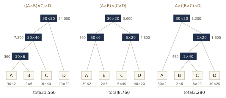
How many trees are there? A tree over \(n\) leaves is a choice of the root’s split point \(k\) together with a tree over the first \(k\) leaves and a tree over the other \(n - k\). The counts are the Catalan numbers, \(\frac{1}{n}\binom{2n-2}{n-1}\) for \(n\) leaves, which grow roughly like \(4^n\):
for n in [4, 8, 16, 32]:
    print(f"{n:2d} matrices: {math.comb(2 * n - 2, n - 1) // n:,} parenthesizations")
 4 matrices: 5 parenthesizations
 8 matrices: 429 parenthesizations
16 matrices: 9,694,845 parenthesizations
32 matrices: 14,544,636,039,226,909 parenthesizations
Trying them all is out of the question beyond a dozen matrices.
Subproblems on intervals
The trees suggest the subproblems. If a tree is optimal, its two subtrees must be optimal for the products they compute (otherwise swap in cheaper subtrees). The subtrees compute products of contiguous runs of matrices, \(A_i \times A_{i+1} \times \dots \times A_j\). So for a product \(A_1 \times \dots \times A_n\) where \(A_k\) has dimensions \(m_{k-1} \times m_k\), define for \(1 \le i \le j \le n\)
\[C(i, j) = \text{the minimum cost of computing } A_i \times A_{i+1} \times \dots \times A_j.\]A single matrix costs nothing: \(C(i, i) = 0\). For \(i < j\), the root of the optimal tree splits the product after some \(A_k\) with \(i \le k \le j - 1\). The two halves cost \(C(i, k)\) and \(C(k+1, j)\), and they produce matrices of dimensions \(m_{i-1} \times m_k\) and \(m_k \times m_j\), whose product costs \(m_{i-1} m_k m_j\). Try every split:
\[C(i, j) = \min_{i \le k \le j-1} \bigl\{ C(i, k) + C(k+1, j) + m_{i-1} m_k m_j \bigr\}.\]Each subproblem depends only on shorter intervals, so we solve them in order of the interval length \(s = j - i\): first all products of two matrices, then of three, and so on. Recording the best split for each interval lets us rebuild the tree.
def chain_order(m):
    """Cheapest way to compute A_1 x ... x A_n, where A_k is m[k-1] x m[k].
    Returns the minimum number of multiplications and a parenthesization."""
    n = len(m) - 1
    C = [[0] * (n + 1) for _ in range(n + 1)]
    split = [[None] * (n + 1) for _ in range(n + 1)]
    for s in range(1, n):                     # s = j - i, the size of the subproblem
        for i in range(1, n - s + 1):
            j = i + s
            C[i][j] = math.inf
            for k in range(i, j):
                cost = C[i][k] + C[k + 1][j] + m[i - 1] * m[k] * m[j]
                if cost < C[i][j]:
                    C[i][j], split[i][j] = cost, k
    def paren(i, j):
        if i == j:
            return NAMES[i - 1]
        k = split[i][j]
        return "(" + paren(i, k) + "×" + paren(k + 1, j) + ")"
    return C[1][n], paren(1, n)

print(chain_order([30, 2, 6, 40, 20]))
(3280, '(A×((B×C)×D))')
The dynamic program finds the order \(A \times ((B \times C) \times D)\) with cost 3,280, the cheapest one in the list above. A randomized check against the exhaustive all_orders:
random.seed(6)
for _ in range(200):
    dims = [random.randint(1, 30) for _ in range(random.randint(2, 8))]
    cost, order = chain_order(dims)
    assert cost == min(c for c, _ in all_orders(dims, 1, len(dims) - 1))
    assert (cost, order) in set(all_orders(dims, 1, len(dims) - 1))
print("200 random chains of 1 to 7 matrices: chain_order is optimal")
200 random chains of 1 to 7 matrices: chain_order is optimal
The second assertion checks that the reconstructed parenthesization really has the reported cost. Running time: there are \(O(n^2)\) subproblems \((i, j)\), and each takes \(O(j - i) = O(n)\) time to minimize over the split points, so the total is \(O(n^3)\). (Summing more carefully gives about \(n^3/6\) inner steps, so the bound is tight.)
Shortest paths
We began with shortest paths in DAGs. Dynamic programming also handles shortest-path problems on general graphs, provided we choose subproblems that carry the right extra information.
Shortest reliable paths
In a communication network, each extra hop on a route is another chance for a packet to be lost. So we may want not just a short route, but a short route with few edges. Given a directed graph with edge lengths, nodes \(s\) and \(t\), and an integer \(k\), find the shortest path from \(s\) to \(t\) that uses at most \(k\) edges.
Dijkstra’s algorithm cannot be adapted directly: it keeps only the length of the best path found to each node and forgets how many edges that path used, which is now essential. The dynamic-programming fix is to put the missing information into the subproblem. For each node \(v\) and each \(i = 0, 1, \dots, k\) let
\[\text{dist}(v, i) = \text{the length of the shortest path from } s \text{ to } v \text{ that uses at most } i \text{ edges}.\]With zero edges only \(s\) is reachable: \(\text{dist}(s, 0) = 0\) and \(\text{dist}(v, 0) = \infty\) for \(v \ne s\). A path with at most \(i\) edges either uses at most \(i - 1\), or ends with an edge \((u, v)\) after a path with at most \(i - 1\) edges to \(u\):
\[\text{dist}(v, i) = \min\Bigl\{ \text{dist}(v, i-1),\ \ \min_{(u, v) \in E} \bigl\{\text{dist}(u, i-1) + \ell(u, v)\bigr\} \Bigr\}.\]The subproblems are ordered by \(i\). Here is a small network where the shortest path from s to t uses four edges, and shorter hop counts cost more:
network = {
    "s": [("a", 1), ("d", 4)],
    "a": [("b", 2), ("d", 2)],
    "b": [("c", 1)],
    "c": [("t", 1)],
    "d": [("t", 3)],
    "t": [],
}

def shortest_path_at_most_k(graph, s, t, k):
    """Length and nodes of a shortest s-t path with at most k edges
    (math.inf, None if there is none)."""
    pred = predecessors(graph)
    dist = [{v: math.inf for v in graph}]
    dist[0][s] = 0
    via = [{}]      # via[i][v] = u if the best path with <= i edges ends with (u, v)
    for i in range(1, k + 1):
        d, before, choice = {}, dist[i - 1], {}
        for v in graph:
            d[v] = before[v]                          # at most i - 1 edges
            for u, w in pred[v]:
                if before[u] + w < d[v]:
                    d[v], choice[v] = before[u] + w, u
        dist.append(d)
        via.append(choice)
    if dist[k][t] == math.inf:
        return math.inf, None
    path, v = [t], t
    for i in range(k, 0, -1):                         # walk back one layer at a time
        if v in via[i]:
            v = via[i][v]
            path.append(v)
    return dist[k][t], path[::-1]

for k in range(1, 5):
    print(f"k = {k}:", shortest_path_at_most_k(network, "s", "t", k))
k = 1: (inf, None)
k = 2: (7, ['s', 'd', 't'])
k = 3: (6, ['s', 'a', 'd', 't'])
k = 4: (5, ['s', 'a', 'b', 'c', 't'])
With one edge there is no path; allowing more edges gives successively shorter routes, down to the true shortest path of length 5 with four edges. The table has \((k+1)\) layers of \(\lvert V \rvert\) entries, and building layer \(i\) looks at every edge once, so the running time is \(O(k(\lvert V \rvert + \lvert E \rvert))\).
Note. With \(k = \lvert V \rvert - 1\) the restriction disappears (a shortest path in a graph without negative cycles never needs more edges than that), and the computation becomes the Bellman–Ford algorithm from module 04: each layer is one round of updating every edge. Bellman–Ford was a dynamic program all along; its subproblems are “shortest path using at most \(i\) edges”.
All-pairs shortest paths: Floyd–Warshall
Now we want the shortest-path distance between every pair of nodes, and edge lengths may be negative (but there is no negative cycle). One option is to run Bellman–Ford from every node, for \(O(\lvert V \rvert^2 \lvert E \rvert)\) time, which is \(O(\lvert V \rvert^4)\) for dense graphs. A cleverer choice of subproblem gives \(O(\lvert V \rvert^3)\).
Number the nodes \(1, \dots, n\). A shortest path from \(i\) to \(j\) passes through some intermediate nodes (all nodes on it except the two ends). Restrict which nodes may be intermediates, and relax the restriction one node at a time:
\[\text{dist}(i, j, k) = \text{the length of the shortest path from } i \text{ to } j \text{ whose intermediate nodes all lie in } \{1, \dots, k\}.\]With \(k = 0\) no intermediates are allowed, so \(\text{dist}(i, j, 0)\) is the length of the edge \((i, j)\) if there is one, \(\infty\) otherwise (and 0 when \(i = j\)). With \(k = n\) every path is allowed, and we have the answers.
What changes when node \(k\) becomes available? A shortest path from \(i\) to \(j\) with intermediates in \(\{1, \dots, k\}\) either avoids \(k\) — then it is the old answer \(\text{dist}(i, j, k-1)\) — or passes through \(k\) exactly once (with no negative cycles, repeating a node never helps). In the second case it splits into a piece from \(i\) to \(k\) and a piece from \(k\) to \(j\), each with intermediates in \(\{1, \dots, k-1\}\):
\[\text{dist}(i, j, k) = \min\bigl\{ \text{dist}(i, j, k-1),\ \ \text{dist}(i, k, k-1) + \text{dist}(k, j, k-1) \bigr\}.\]There are \(n^3\) subproblems, each solved in constant time. And we do not need a three-dimensional table: going from \(k-1\) to \(k\) never changes the entries in row \(k\) or column \(k\) (a path from \(i\) to \(k\) gains nothing by using \(k\) as an intermediate too), so we can update a single \(n \times n\) matrix in place. For path recovery we keep a second matrix, nxt[i][j], the node that follows \(i\) on the best path found so far to \(j\).
def floyd_warshall(graph):
    """All-pairs shortest paths. graph: {u: [(v, length), ...]} with nodes 0 .. n-1.
    Returns (dist, nxt): dist[i][j] is the distance from i to j,
    and nxt[i][j] the node after i on a shortest path."""
    n = len(graph)
    dist = [[0 if i == j else math.inf for j in range(n)] for i in range(n)]
    nxt = [[i if i == j else None for j in range(n)] for i in range(n)]
    for u in graph:
        for v, w in graph[u]:
            if w < dist[u][v]:
                dist[u][v], nxt[u][v] = w, v
    for k in range(n):                   # allow node k as an intermediate
        for i in range(n):
            if dist[i][k] == math.inf:
                continue
            for j in range(n):
                if dist[i][k] + dist[k][j] < dist[i][j]:
                    dist[i][j] = dist[i][k] + dist[k][j]
                    nxt[i][j] = nxt[i][k]
    return dist, nxt

def fw_path(nxt, i, j):
    """The nodes of a shortest path from i to j, read off the nxt matrix."""
    if nxt[i][j] is None:
        return None
    path = [i]
    while i != j:
        i = nxt[i][j]
        path.append(i)
    return path

g = {0: [(1, 4), (2, 1)], 1: [(3, 1)], 2: [(1, -2), (3, 5)], 3: [(0, 2)]}
dist, nxt = floyd_warshall(g)
for row in dist:
    print(" ".join(f"{d:>3}" for d in row))
print("shortest path from 0 to 3:", fw_path(nxt, 0, 3))
  0  -1   1   0
  3   0   4   1
  1  -2   0  -1
  2   1   3   0
shortest path from 0 to 3: [0, 2, 1, 3]
The negative edge \(2 \to 1\) makes the best route from 0 to 3 go the long way around, through 2 and 1, for a total length of 0.
To test it, we compare against Bellman–Ford run from every node, on random graphs with some negative edges. A random graph may contain a negative cycle, in which case shortest paths are not defined; Floyd–Warshall reveals this with a negative entry on the diagonal (a path from a node back to itself of negative length), and we skip those graphs.
def bellman_ford(graph, s):
    """Distances from s; negative edges allowed, negative cycles not. n - 1 rounds."""
    dist = {u: math.inf for u in graph}
    dist[s] = 0
    for _ in range(len(graph) - 1):
        for u in graph:
            for v, w in graph[u]:
                if dist[u] + w < dist[v]:
                    dist[v] = dist[u] + w
    return dist

random.seed(7)
checked = skipped = 0
for _ in range(300):
    n = random.randint(2, 8)
    graph = {u: [(v, random.randint(-2, 9)) for v in range(n)
                 if v != u and random.random() < 0.4]
             for u in range(n)}
    dist, nxt = floyd_warshall(graph)
    if any(dist[i][i] < 0 for i in range(n)):
        skipped += 1
        continue
    for s in range(n):
        bf = bellman_ford(graph, s)
        assert all(dist[s][t] == bf[t] for t in range(n))
        for t in range(n):
            p = fw_path(nxt, s, t)
            length = sum(dict(graph[a])[b] for a, b in zip(p, p[1:])) if p else math.inf
            assert length == dist[s][t]
    checked += 1
print(f"{checked} graphs agree with Bellman-Ford from every node")
print(f"{skipped} graphs skipped because they have a negative cycle")
245 graphs agree with Bellman-Ford from every node
55 graphs skipped because they have a negative cycle
The three nested loops make the running time \(O(\lvert V \rvert^3)\), and memory is \(O(\lvert V \rvert^2)\) for the two matrices. With nonnegative lengths, running Dijkstra’s algorithm from every node takes \(O(\lvert V \rvert (\lvert V \rvert + \lvert E \rvert) \log \lvert V \rvert)\), which is better for sparse graphs; Floyd–Warshall wins on dense graphs, handles negative edges, and its core is a triple loop of a few lines.
Watch out. Floyd–Warshall’s recurrence assumes there is no negative cycle: the claim that a shortest path visits node \(k\) at most once fails otherwise. The algorithm still terminates, and a negative cycle shows up as some \(\text{dist}(i, i) < 0\) at the end — check the diagonal before trusting the other entries.
The traveling salesman problem
A salesperson must start from home, visit each of \(n - 1\) other cities exactly once, and return home. Given the distances \(d_{ij}\) between all pairs of cities, which tour is shortest? This is the traveling salesman problem (TSP), one of the most studied problems in computing. Here is a five-city instance, with city 0 as home:
D = [[0, 3, 4, 2, 7],
     [3, 0, 4, 6, 3],
     [4, 4, 0, 5, 8],
     [2, 6, 5, 0, 6],
     [7, 3, 8, 6, 0]]
Brute force tries all \((n-1)!\) orders of the other cities, which takes \(O(n!)\) time. Dynamic programming does much better, though still exponentially: as we will see in module 07, a polynomial-time algorithm for the TSP is very unlikely to exist.
Subproblems. Think of building a tour one city at a time. To extend a partial tour, what must we know? The city \(j\) where we currently are, since it determines the cost of the next step, and the set of cities visited so far, so that we do not repeat any; the order in which we visited them no longer matters. So for every set \(S\) of cities that contains the home city and every \(j \in S\), let
\[C(S, j) = \text{the length of the shortest path that starts at the home city, visits each city of } S \text{ exactly once, and ends at } j.\]Number the home city 0, as in the code. The base case is \(C(\{0\}, 0) = 0\), and for \(S\) with more than one city we set \(C(S, 0) = \infty\), since such a path cannot both start and end at home. For \(j \ne 0\), the path’s second-to-last city is some \(i \in S\) with \(i \ne j\), and the path up to \(i\) must be the shortest one through \(S \setminus \{j\}\):
\[C(S, j) = \min_{i \in S,\ i \ne j} \bigl\{ C(S \setminus \{j\}, i) + d_{ij} \bigr\}.\]Finally, the best tour closes the loop: its length is \(\min_{j} \{C(\{0, \dots, n-1\}, j) + d_{j0}\}\).
The subproblems can be solved in order of increasing \(\lvert S \rvert\). In code, we represent a set \(S\) of cities as an integer bitmask: bit \(j\) is 1 when city \(j\) is in \(S\). Removing \(j\) from \(S\) is S ^ (1 << j), which is numerically smaller than S, so processing the masks in increasing numeric order is also a valid order.
def tsp(d):
    """Shortest tour through all cities of distance matrix d, from and back to city 0.
    Returns (length, tour)."""
    n = len(d)
    C = [[math.inf] * n for _ in range(1 << n)]      # C[S][j]
    parent = [[None] * n for _ in range(1 << n)]
    C[1][0] = 0                                      # S = {0}, standing at city 0
    for S in range(1, 1 << n, 2):             # odd masks: the sets that contain city 0
        for j in range(1, n):
            if not S & (1 << j):
                continue
            rest = S ^ (1 << j)                      # S without j
            for i in range(n):
                if rest & (1 << i) and C[rest][i] + d[i][j] < C[S][j]:
                    C[S][j], parent[S][j] = C[rest][i] + d[i][j], i
    full = (1 << n) - 1
    length, j = min((C[full][j] + d[j][0], j) for j in range(1, n))
    tour, S = [], full
    while j is not None:                             # walk the parents back to city 0
        tour.append(j)
        S, j = S ^ (1 << j), parent[S][j]
    return length, tour[::-1] + [0]

tsp(D)
(19, [0, 3, 4, 1, 2, 0])
The optimal tour has length 19. For comparison, the greedy “nearest neighbor” rule — always go to the closest unvisited city — gives the tour 0, 3, 2, 1, 4, 0 of length 21 on this instance. Against brute force over all permutations, for up to eight cities:
from itertools import permutations

def tsp_brute(d):
    """Length of the shortest tour, trying all (n-1)! orders of cities 1 .. n-1."""
    n = len(d)
    return min(sum(d[a][b] for a, b in zip((0,) + p, p + (0,)))
               for p in permutations(range(1, n)))

random.seed(8)
for n in range(2, 9):
    for _ in range(4):
        d = [[0] * n for _ in range(n)]
        for a, b in combinations(range(n), 2):
            d[a][b] = d[b][a] = random.randint(1, 20)
        length, tour = tsp(d)
        assert length == tsp_brute(d)
        assert sorted(tour[:-1]) == list(range(n)) and tour[0] == tour[-1] == 0
        assert length == sum(d[a][b] for a, b in zip(tour, tour[1:]))
print("random instances with 2 to 8 cities: tsp agrees with brute force")
random instances with 2 to 8 cities: tsp agrees with brute force
Running time. There are at most \(2^n \cdot n\) subproblems \((S, j)\), and each takes \(O(n)\) time, so the total is \(O(n^2 2^n)\); memory is \(O(n 2^n)\). That is still exponential, but far smaller than \((n-1)!\):
for n in [10, 15, 20, 25]:
    print(f"n = {n}: (n-1)! = {math.factorial(n - 1):.2e}   n^2 2^n = {n**2 * 2**n:.2e}")
n = 10: (n-1)! = 3.63e+05   n^2 2^n = 1.02e+05
n = 15: (n-1)! = 8.72e+10   n^2 2^n = 7.37e+06
n = 20: (n-1)! = 1.22e+17   n^2 2^n = 4.19e+08
n = 25: (n-1)! = 6.20e+23   n^2 2^n = 2.10e+10
At 20 cities, brute force is hopeless while the dynamic program needs a few hundred million steps. Memory, \(n 2^n\) table entries, is usually what stops it.
Independent sets in trees
A set of nodes \(I\) in an undirected graph is an independent set if no edge joins two nodes of \(I\). Finding a largest independent set in a general graph is another problem for which no polynomial-time algorithm is known (module 07). But when the graph is a tree, dynamic programming solves it in linear time.
Subproblems. Pick any node \(r\) as the root. Every node \(u\) then has a subtree hanging from it: \(u\) together with all its descendants. Let
\[I(u) = \text{the size of a largest independent set in the subtree hanging from } u.\]The answer is \(I(r)\). A largest independent set of \(u\)’s subtree either contains \(u\) or it does not. If it does, none of \(u\)’s children can be in it, but the subtrees of \(u\)’s grandchildren are unconstrained. If it does not, the subtrees of \(u\)’s children are unconstrained. So
\[I(u) = \max\Bigl\{ 1 + \sum_{w \text{ a grandchild of } u} I(w),\ \ \sum_{w \text{ a child of } u} I(w) \Bigr\}.\]For a leaf, both sums are empty and \(I(u) = 1\). The subproblems are solved from the leaves up, children before parents; any order where each node comes after all its descendants will do, such as the reverse of the order in which a search from the root discovers the nodes.
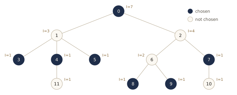
The tree is stored as undirected adjacency lists. The code finds each node’s parent with an iterative search from the root, computes \(I\) bottom-up, and then walks down from the root to recover a set, taking a node exactly when the recurrence chose the “contains \(u\)” option there.
def tree_independent_set(tree, root):
    """Largest independent set of a tree given as adjacency lists {u: [v, ...]}.
    Returns (size, set of nodes)."""
    parent, order, stack = {root: None}, [], [root]
    while stack:                     # order: every parent comes before its children
        u = stack.pop()
        order.append(u)
        for v in tree[u]:
            if v != parent[u]:
                parent[v] = u
                stack.append(v)
    children = {u: [v for v in tree[u] if v != parent[u]] for u in tree}
    I, take = {}, {}
    for u in reversed(order):        # every node after all its descendants
        with_u = 1 + sum(I[g] for c in children[u] for g in children[c])
        without_u = sum(I[c] for c in children[u])
        I[u], take[u] = max(with_u, without_u), with_u >= without_u
    chosen, stack = set(), [root]
    while stack:                     # walk down, following the choices made
        u = stack.pop()
        if take[u]:
            chosen.add(u)
            stack.extend(g for c in children[u] for g in children[c])
        else:
            stack.extend(children[u])
    return I[root], chosen

edges = [(0, 1), (0, 2), (1, 3), (1, 4), (1, 5), (2, 6), (2, 7),
         (4, 11), (6, 8), (6, 9), (7, 10)]
tree = {u: [] for u in range(12)}
for a, b in edges:
    tree[a].append(b)
    tree[b].append(a)
size, chosen = tree_independent_set(tree, 0)
print(size, sorted(chosen))
7 [0, 3, 4, 5, 7, 8, 9]
The result matches the figure. To check it, we compare with a brute-force search over all subsets of nodes, on random trees of up to 12 nodes (each new node attaches to a random earlier one):
def independent_set_brute(n, edges):
    """Size of a largest independent set, by trying all subsets of {0, ..., n-1}."""
    return max(len(S) for k in range(n + 1) for S in map(set, combinations(range(n), k))
               if not any(a in S and b in S for a, b in edges))

random.seed(9)
for _ in range(100):
    n = random.randint(1, 12)
    edges = [(random.randrange(v), v) for v in range(1, n)]
    tree = {u: [] for u in range(n)}
    for a, b in edges:
        tree[a].append(b)
        tree[b].append(a)
    size, chosen = tree_independent_set(tree, random.randrange(n))
    assert size == len(chosen) == independent_set_brute(n, edges)
    assert not any(a in chosen and b in chosen for a, b in edges)
print("100 random trees: tree_independent_set agrees with brute force")
100 random trees: tree_independent_set agrees with brute force
The random root in the test is deliberate: the answer must not depend on which node we root the tree at.
Running time. There is one subproblem per node. Computing \(I(u)\) reads the values of \(u\)’s children and grandchildren, and each node is read at most twice in total — once by its parent and once by its grandparent — so all the sums together take \(O(\lvert V \rvert)\) time. Finding parents and the order is a graph search, \(O(\lvert V \rvert + \lvert E \rvert)\), which for a tree is \(O(\lvert V \rvert)\) as well. The whole algorithm is linear.
Summary
| Problem | Subproblems | Number of subproblems | Running time |
|---|---|---|---|
| shortest or longest path in a DAG | \(\text{dist}(v)\) for each node | \(\lvert V \rvert\) | \(O(\lvert V \rvert + \lvert E \rvert)\) |
| longest increasing subsequence | \(L(j)\): longest one ending at \(j\) | \(n\) | \(O(n^2)\) |
| edit distance | \(E(i, j)\): pairs of prefixes | \((m+1)(n+1)\) | \(O(mn)\) |
| knapsack with repetition | \(K(w)\): smaller capacities | \(W + 1\) | \(O(nW)\), pseudo-polynomial |
| knapsack without repetition | \(K(w, j)\): capacity and first \(j\) items | \((W+1)(n+1)\) | \(O(nW)\), pseudo-polynomial |
| chain matrix multiplication | \(C(i, j)\): intervals of the chain | \(O(n^2)\) | \(O(n^3)\) |
| shortest path with at most \(k\) edges | \(\text{dist}(v, i)\) | \((k+1)\lvert V \rvert\) | \(O(k(\lvert V \rvert + \lvert E \rvert))\) |
| all-pairs shortest paths (Floyd–Warshall) | \(\text{dist}(i, j, k)\): intermediates in \(\{1, \dots, k\}\) | \(\lvert V \rvert^3\) | \(O(\lvert V \rvert^3)\) |
| traveling salesman | \(C(S, j)\): set visited, current city | \(O(n 2^n)\) | \(O(n^2 2^n)\) |
| independent set in a tree | \(I(u)\): subtree hanging from \(u\) | \(\lvert V \rvert\) | \(O(\lvert V \rvert)\) |
Ideas to carry forward:
- A dynamic program is a set of subproblems, a recurrence, and an order. The subproblems and their dependencies form a DAG; the running time is roughly the number of edges in it, and memory can often be recycled once a subproblem’s dependents are done.
- The creative step is choosing subproblems. Ask what you must remember about a partial solution to extend it — a prefix, a pair of prefixes, an interval, a subtree, a remaining capacity, a set of visited cities — and make that the subproblem’s parameters.
- Correctness rests on optimal substructure: an optimal solution is assembled from optimal solutions to subproblems, which a cut-and-paste argument proves.
- Recover the solution itself, not just its value, by recording each choice and walking the choices back. Solve each subproblem once, bottom-up or with memoization; plain recursion on the recurrence is usually exponential.
Exercises
- Best contiguous block. Given numbers \(a_1, \dots, a_n\) (some negative), find a contiguous block \(a_i, \dots, a_j\) with the largest sum (the empty block has sum 0). Define \(B(j)\) as the best sum of a block ending at \(j\), write a recurrence, and give an \(O(n)\) algorithm. Implement it and test it against an \(O(n^2)\) brute force on random lists.
- Faster increasing subsequences. Scan the sequence left to right, maintaining for each length \(\ell\) the smallest value that ends an increasing subsequence of length \(\ell\) seen so far. Prove that these values are strictly increasing in \(\ell\), and use this to process each new element with one binary search (
bisect.bisect_left), for \(O(n \log n)\) total. Test your code againstlis. - Longest common subsequence. A common subsequence of \(x\) and \(y\) is a sequence that is a subsequence of both. Give an \(O(mn)\) dynamic program for the length of a longest common subsequence, with a recurrence on pairs of prefixes, and recover one such subsequence. Then show that if only insertions and deletions are allowed (no substitutions), the minimum number of edits turning \(x\) into \(y\) is \(m + n - 2\,\text{LCS}(x, y)\).
- Weighted edits. Modify
edit_distance_tableso that an insertion costs \(c_I\), a deletion \(c_D\), and a substitution \(c_S\). What happens to the optimal alignments when \(c_S > c_I + c_D\)? In the DAG view, which edge lengths change? - Why the second index? Give a concrete instance (weights, values, capacity) on which the one-index recurrence \(K(w) = \max_i \{K(w - w_i) + v_i\}\) returns more than the best knapsack without repetition, and say what information \(K(w)\) fails to record. Then prove the recurrence for \(K(w, j)\) correct by the cut-and-paste argument.
- Making change. Coins come in denominations \(c_1, \dots, c_n\), with an unlimited supply of each. (a) Give an \(O(nv)\) algorithm that decides whether an amount \(v\) can be paid exactly. (b) Give an \(O(nv)\) algorithm for the fewest coins needed. (c) Count the number of different multisets of coins that pay \(v\), and explain why your loop order counts {1, 2} and {2, 1} once. Is \(O(nv)\) polynomial?
- Counting parenthesizations. Let \(P(n)\) be the number of ways to parenthesize a product of \(n\) matrices. Show \(P(1) = 1\) and \(P(n) = \sum_{k=1}^{n-1} P(k) P(n-k)\), and prove \(P(n) \ge 2^{n-2}\) for \(n \ge 2\). Then find (by hand or by a search with
chain_order) dimensions for which the rule “split at the smallest inner dimension \(m_k\)” is not optimal. - Floyd–Warshall details. (a) Prove that during iteration \(k\) the entries \(\text{dist}[i][k]\) and \(\text{dist}[k][j]\) do not change, which justifies updating a single matrix in place. (b) Prove that if the graph has a negative cycle, some diagonal entry is negative when the algorithm stops. (c) Adapt the algorithm to compute, for every pair, whether any path exists (the transitive closure), using only Boolean operations.
- Paths instead of tours. Modify
tspto find the shortest path that visits every city exactly once, starting at city 0 and ending anywhere. Then modify it again so that the start is also free. What are the running times? - Two values per node. Rewrite
tree_independent_setwith two values per node: \(\text{in}(u)\), the largest independent set of \(u\)’s subtree that contains \(u\), and \(\text{out}(u)\), the largest that does not. Write both recurrences using children only. Then solve the weighted version, where each node has a positive weight and we maximize total weight, and test it against brute force. - Memoization depth. Call
knapsack_rep_memo(5000, [1, 2], [1, 3]). What happens, and why? Explain whylis_length_topdownon a sorted list of length 5,000 does not run into the same problem, even though its subproblem DAG is just as deep. (Hint: in what order does it make its recursive calls?) Then fixknapsack_rep_memowithout giving up the dictionary, so that the recursion never goes more than a few levels deep. - In your own words: explain to a classmate how dynamic programming differs from divide and conquer, and why a recursive solution to the recurrence for \(L(j)\) is exponential while one for mergesort is not. Then describe one situation where top-down memoization is the better choice and one where a bottom-up table is.
Going further
- Dasgupta, Papadimitriou, and Vazirani, Algorithms, chapter 6 — the source for this module. Good practice: exercises 6.1, 6.2, 6.11, 6.17–6.19 (variants of knapsack and change-making), 6.20 (optimal binary search trees), 6.21 (vertex cover in trees), and 6.26–6.28 (sequence alignment).
- Robert A. Wagner and Michael J. Fischer, “The string-to-string correction problem”, Journal of the ACM, 1974 — the edit-distance dynamic program.
- Robert W. Floyd, “Algorithm 97: Shortest path”, Communications of the ACM, 1962 — the all-pairs algorithm in a few lines.
- Michael Held and Richard M. Karp, “A dynamic programming approach to sequencing problems”, Journal of SIAM, 1962 — the \(O(n^2 2^n)\) algorithm for the traveling salesman problem.
- Jeff Erickson, Algorithms, chapter 3 (Dynamic Programming) — a free textbook with many more worked examples and exercises; its treatment of edit distance also discusses the linear-space alignment method.
- Python documentation:
functools.cache.
These notes follow the chapters of S. Dasgupta, C. H. Papadimitriou, and U. V. Vazirani, Algorithms (McGraw-Hill, 2008), the course text. The explanations, code, figures, and exercises here are written for this course; the book remains the reference, with many more exercises.