CSE 431/531 · Module 00 · Week 1
Prologue: Why Algorithms, and Big-O
Two ways to compute Fibonacci numbers, the three questions we ask of every algorithm, and big-O notation.
Companion reading: Dasgupta, Papadimitriou & Vazirani, Algorithms, chapter 0, “Prologue”
By the end of this module you can
- Ask the three questions of any algorithm — is it correct, how long does it take, can we do better — and answer them for a short procedure.
- Write a recurrence for the running time of a recursive algorithm and use it to show that the running time is exponential.
- Explain why storing intermediate results turns an exponential algorithm into a polynomial one.
- Account for the size of the numbers when you count the steps an algorithm takes.
- Define \(O\), \(\Omega\), and \(\Theta\) precisely, and prove or disprove a claim such as \(f = O(g)\) by finding, or ruling out, a constant.
- Rank logarithmic, polynomial, and exponential running times, and estimate what input sizes each can handle.
Contents
- What an algorithm is
- Fibonacci numbers
- A first algorithm: follow the definition
- A better algorithm: remember what you computed
- Counting more carefully: the size of the numbers
- Can we do better? Powers of a matrix
- Big-O notation
- Summary
- Exercises
- Going further
This course is about a single skill: given a computational problem, find a procedure that solves it, convince yourself (and others) that it is right, and say precisely how its cost grows with the size of the input. The rest of the term applies that skill to numbers, graphs, strings, and optimization problems, using a handful of design strategies — divide and conquer, greedy choice, dynamic programming — and ends by asking which problems have no efficient algorithm at all.
This first module sets up the vocabulary. We look at one small problem, computing Fibonacci numbers, and find that the obvious algorithm is hopelessly slow while a slightly less obvious one is fast. Then we introduce big-O notation, the language we use for the rest of the course to talk about running time without drowning in detail.
What an algorithm is
An algorithm is a finite, precise, step-by-step procedure for solving a problem: every step is unambiguous, it can be carried out mechanically, and it stops with the right answer on every valid input. The word comes from the name of al-Khwarizmi, a ninth-century scholar in Baghdad whose book on the Hindu–Arabic decimal system taught generations of readers how to add, multiply, and divide numbers written in positional notation. Those procedures are algorithms in exactly our sense, and the reason they spread is the reason we study algorithms at all: a good procedure makes a hard task routine.
The same problem usually has many algorithms, and they can differ enormously in cost. That difference, more than raw hardware speed, decides what is practical to compute. The Fibonacci example below makes the point with a factor that is not 2 or 10 but astronomically large.
Note. The notes write algorithms in Python. Python is close enough to the pseudocode used in the textbook that you can read it the same way, and it lets you run everything. Each code block shows its real output underneath, in a box labeled Output. Type the examples yourself and change them; the best way to understand a running-time claim is to test it.
Fibonacci numbers
The Fibonacci numbers start with 0 and 1, and each later number is the sum of the two before it:
\[F_n = \begin{cases} 0 & \text{if } n = 0, \\ 1 & \text{if } n = 1, \\ F_{n-1} + F_{n-2} & \text{if } n > 1. \end{cases}\]The sequence begins 0, 1, 1, 2, 3, 5, 8, 13, 21, 34, and it grows quickly: \(F_{30}\) is already more than 800,000. After the powers of 2, it is probably the sequence computer scientists meet most often, and it is a convenient test case because the definition is a recipe you can follow directly. Our problem is:
Given a non-negative integer \(n\), compute \(F_n\).
A first algorithm: follow the definition
The definition is recursive, so the most direct algorithm is a recursive function that says the same thing.
def fib1(n):
    """F(n) straight from the definition."""
    if n == 0:
        return 0
    if n == 1:
        return 1
    return fib1(n - 1) + fib1(n - 2)

[fib1(n) for n in range(11)]
[0, 1, 1, 2, 3, 5, 8, 13, 21, 34, 55]
Whenever we meet an algorithm, we ask three questions, in this order:
- Is it correct? Does it return the right answer on every valid input?
- How long does it take, as a function of the input?
- Can we do better?
For fib1 the first question is easy: the code is the definition, so it returns \(F_n\) for every \(n \ge 0\). (Strictly, we argue by induction on \(n\): the two base cases are right, and if the calls on \(n-1\) and \(n-2\) return the right values, so does the call on \(n\).) The second question is where the trouble is.
How long does it take?
Let \(T(n)\) be the number of basic steps fib1(n) performs. For now, count each comparison, return, and addition as one step; we revisit that assumption later in this module. When \(n \le 1\) the function does at most two steps, so \(T(n) \le 2\). When \(n > 1\) it makes two recursive calls, which cost \(T(n-1)\) and \(T(n-2)\), plus a few steps of its own — two comparisons and one addition:
A formula that defines a function in terms of its own values at smaller inputs is a recurrence. Compare this one with the recurrence for \(F_n\): it has the same shape, with an extra \(+3\) each time. So \(T(n) \ge F_n\) for every \(n\) (check the base cases, then induct). The running time of fib1 grows at least as fast as the Fibonacci numbers themselves.
How fast is that? Since \(F_{n-1} \ge F_{n-2}\), we have \(F_n = F_{n-1} + F_{n-2} \ge 2F_{n-2}\): the sequence at least doubles every two steps. That gives \(F_n \ge 2^{n/2}\) for \(n \ge 6\), and a more careful calculation shows \(F_n \approx 2^{0.694n}\). Exponential growth in the answer means exponential growth in the running time.
We can watch this happen by counting calls instead of reading a clock. Counting is exact and does not depend on the machine.
def count_calls(n):
    """Number of calls fib1(n) makes, including the first one."""
    if n <= 1:
        return 1
    return 1 + count_calls(n - 1) + count_calls(n - 2)

for n in [10, 20, 30]:
    print(f"n = {n:2d}   F(n) = {fib1(n):7d}   calls = {count_calls(n):9,d}")
n = 10   F(n) =      55   calls =       177
n = 20   F(n) =    6765   calls =    21,891
n = 30   F(n) =  832040   calls = 2,692,537
Adding 10 to \(n\) multiplies the work by about 123, and \(1.618^{10} \approx 123\). The recursion tree shows where all those calls come from.
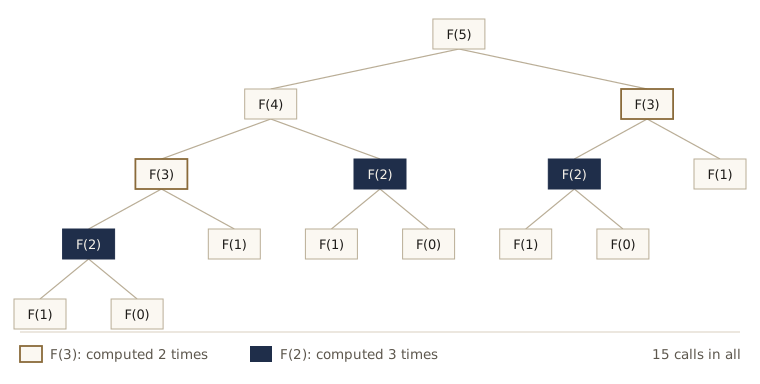
fib1(5). The same subproblems are solved over and over: fib1(3) twice, fib1(2) three times, fib1(1) five times. The repetition grows exponentially with n.What exponential time means in practice
Now the clock. Each call is fast, but there are so many of them that even modest inputs take a noticeable time.
import time

for n in [24, 28, 32]:
    start = time.perf_counter()
    fib1(n)
    print(f"fib1({n}) took {time.perf_counter() - start:.3f} s")
fib1(24) took 0.006 s
fib1(28) took 0.039 s
fib1(32) took 0.270 s
Your times will differ, but the ratios will not: each step of 4 in \(n\) costs a factor of about \(1.618^4 \approx 6.9\). Extrapolate, and fib1(100) would take about \(10^{14}\) times as long as fib1(32) — more than a million years. Faster hardware does not rescue us. If computers get about 1.6 times faster every year, that buys exactly one more Fibonacci number per year, because each \(F_{n+1}\) costs about 1.6 times as much as \(F_n\). This is the curse of exponential time: improvements in the machine are swallowed by a tiny increase in the input.
A better algorithm: remember what you computed
The tree above shows the problem: fib1 recomputes the same values again and again. A more sensible procedure computes \(F_0, F_1, F_2, \dots\) in order, and keeps each value as soon as it is known.
def fib2(n):
    """F(n) by filling a table from the bottom up."""
    if n == 0:
        return 0
    f = [0] * (n + 1)
    f[1] = 1
    for i in range(2, n + 1):
        f[i] = f[i - 1] + f[i - 2]
    return f[n]

print([fib2(n) for n in range(11)])
print(fib2(100))
print(fib2(200))
[0, 1, 1, 2, 3, 5, 8, 13, 21, 34, 55]
354224848179261915075
280571172992510140037611932413038677189525
Correctness is again immediate: the loop applies the definition, and each f[i] is filled in only after the two entries it depends on. The running time is different in kind. The loop body runs \(n - 1\) times and does one addition each time, so the number of steps is proportional to \(n\). We have gone from exponential to polynomial (here, linear) time. \(F_{200}\), which fib1 could never reach, takes a fraction of a millisecond.
The same idea can be kept in recursive form: let the recursive function remember the answers it has already returned. This is called memoization, and Python provides it as a decorator.
from functools import cache

@cache
def fib_memo(n):
    if n <= 1:
        return n
    return fib_memo(n - 1) + fib_memo(n - 2)

fib_memo(200) == fib2(200)
True
Note. Solving each subproblem once and storing the result is the central idea of dynamic programming, the subject of module 06. The Fibonacci numbers are its smallest example: the subproblems are \(F_0, \dots, F_{n-1}\), and each depends on the two before it.
Counting more carefully: the size of the numbers
So far we have treated an addition as one step. That is reasonable for numbers that fit in a machine word — 64 bits, say — but Fibonacci numbers do not stay that small. Python’s integers grow as needed, so we can ask how many bits \(F_n\) has.
for n in [100, 1_000, 10_000, 100_000]:
    bits = fib2(n).bit_length()
    print(f"F({n:>6}) has {bits:>6} bits   ({bits / n:.3f} bits per unit of n)")
F(   100) has     69 bits   (0.690 bits per unit of n)
F(  1000) has    694 bits   (0.694 bits per unit of n)
F( 10000) has   6942 bits   (0.694 bits per unit of n)
F(100000) has  69424 bits   (0.694 bits per unit of n)
So \(F_n\) is about \(0.694n\) bits long, which matches \(F_n \approx 2^{0.694n}\). Adding two numbers of that length cannot be a single step. As we will see in module 01, adding two \(k\)-bit numbers takes time proportional to \(k\), just as grade-school addition works one digit at a time. With that correction:
fib2does about \(n\) additions on numbers of up to about \(0.694n\) bits, so its running time is proportional to \(n^2\) — still polynomial.fib1does about \(F_n\) additions, each on numbers of up to \(O(n)\) bits, so its running time is proportional to \(nF_n\) — still exponential.
The conclusion survives, but the lesson is general. The size of the input is measured in bits, and “one step” must be an operation whose cost really is constant. When the numbers involved grow with the input, arithmetic on them has to be counted.
Can we do better? Powers of a matrix
fib2 is linear in the number of additions. Can we use fewer arithmetic operations? Write two consecutive Fibonacci numbers as a vector. One step of the recurrence is a matrix multiplication:
Computing \(F_n\) therefore reduces to raising a \(2 \times 2\) matrix \(X\) to the \(n\)th power, and powers can be computed by repeated squaring: \(X^{8} = ((X^2)^2)^2\) takes three multiplications, not seven. For a general \(n\), square when \(n\) is even and peel off one factor when it is odd:
\[X^n = \begin{cases} \left(X^{n/2}\right)^2 & n \text{ even}, \\ X \cdot X^{n-1} & n \text{ odd}. \end{cases}\]The exponent is at least halved every two steps, so only \(O(\log n)\) matrix multiplications are needed.
def mat_mult(A, B):
    """Product of two 2x2 matrices given as ((a, b), (c, d))."""
    (a, b), (c, d) = A
    (e, f), (g, h) = B
    return ((a * e + b * g, a * f + b * h),
            (c * e + d * g, c * f + d * h))

def mat_power(X, n):
    """X to the n-th power by repeated squaring (n >= 0)."""
    if n == 0:
        return ((1, 0), (0, 1))
    if n % 2 == 0:
        half = mat_power(X, n // 2)
        return mat_mult(half, half)
    return mat_mult(X, mat_power(X, n - 1))

def fib3(n):
    """F(n) as the top-right entry of [[0, 1], [1, 1]] ** n."""
    return mat_power(((0, 1), (1, 1)), n)[0][1]

all(fib3(n) == fib2(n) for n in range(500))
True
So fib3 uses \(O(\log n)\) arithmetic operations where fib2 uses \(O(n)\). But its operations are multiplications of numbers with thousands of bits, and multiplication is more expensive than addition. Whether fib3 actually wins depends on how fast we can multiply large integers — a question we answer in module 02. Python happens to use a faster-than-schoolbook method for very large integers, and the difference shows:
n = 200_000
for f in [fib2, fib3]:
    start = time.perf_counter()
    f(n)
    print(f"{f.__name__}({n:,}) took {time.perf_counter() - start:.3f} s")
fib2(200,000) took 1.141 s
fib3(200,000) took 0.011 s
Watch out. “Fewer operations” is only a better algorithm if the operations cost the same.
fib3wins here because of how Python multiplies big integers; with schoolbook multiplication its advantage shrinks. Exercise 6 asks you to work out the bound.
Big-O notation
Our analysis of fib1 and fib2 already simplified a lot. We counted “basic steps” rather than nanoseconds, because the time a step takes depends on the processor, the memory hierarchy, and even what else the machine is doing, and an analysis that tracked all that would describe one machine and nothing else. The next simplification is to ignore constant factors and lower-order terms. If an algorithm takes \(5n^3 + 4n + 3\) steps, we say it takes time \(O(n^3)\): the \(4n + 3\) becomes irrelevant as \(n\) grows, and the factor 5 changes with the machine anyway.
The definition
Think of \(f(n)\) and \(g(n)\) as running times on inputs of size \(n\): functions from positive integers to positive reals.
Definition. \(f = O(g)\) if there is a constant \(c > 0\) such that \(f(n) \le c \cdot g(n)\) for all \(n\).
Read \(f = O(g)\) as “\(f\) grows no faster than \(g\)”. It is a loose version of \(f \le g\): loose because of the constant \(c\), which lets us say \(10n = O(n)\), and which also absorbs whatever happens at small \(n\). Many books state the definition with “for all \(n \ge n_0\)”; for positive functions the two versions are equivalent, since you can raise \(c\) to cover the finitely many \(n < n_0\).
A worked example. Suppose one algorithm takes \(f_1(n) = n^2\) steps and another takes \(f_2(n) = 4n + 32\).
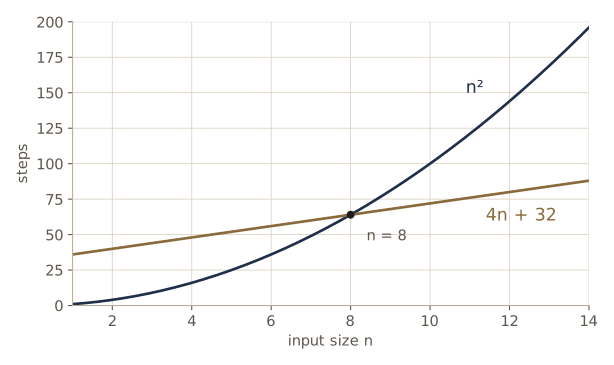
For \(n < 8\) the quadratic one is cheaper, but from \(n = 8\) on the linear one is better, and for large inputs it is better by any factor you like. Big-O captures this:
- \(f_2 = O(f_1)\), because \(\dfrac{f_2(n)}{f_1(n)} = \dfrac{4n + 32}{n^2} \le 36\) for all \(n \ge 1\), so \(c = 36\) works.
- \(f_1 \ne O(f_2)\), because \(\dfrac{f_1(n)}{f_2(n)} = \dfrac{n^2}{4n + 32}\) grows without bound, so no constant \(c\) can work.
Now a third algorithm takes \(f_3(n) = n + 5\) steps. It beats \(f_2\), but only by a constant factor: \(f_2(n)/f_3(n) = (4n+32)/(n+5) \le 6\), so \(f_2 = O(f_3)\), and \(f_3 = O(f_2)\) with \(c = 1\). At the level of big-O, \(f_2\) and \(f_3\) are the same, while \(f_1\) is genuinely worse. That is the distinction we want to keep.
Big-Omega and big-Theta
Big-O is the analog of \(\le\). The analogs of \(\ge\) and \(=\) are:
\[f = \Omega(g) \iff g = O(f), \qquad\qquad f = \Theta(g) \iff f = O(g) \text{ and } f = \Omega(g).\]In the example, \(f_2 = \Theta(f_3)\), and \(f_1 = \Omega(f_3)\) but not \(\Theta(f_3)\). When we know the growth rate exactly, we say so with \(\Theta\); big-O is only an upper bound. Saying “fib2 is \(O(2^n)\)” is true and useless.
Watch out. The “=” in \(f = O(g)\) is not equality: it means “\(f\) belongs to the class of functions that grow no faster than \(g\)”. You can write \(n = O(n^2)\), but \(O(n^2) = n\) is nonsense.
Simplifying expressions
In practice you replace a messy expression by the simplest function with the same growth. For \(3n^2 + 4n + 5\), that is \(n^2\): the quadratic term dominates the rest. These rules cover most cases:
- Drop multiplicative constants: \(14n^2\) becomes \(n^2\).
- Among powers, the larger exponent dominates: \(n^a\) dominates \(n^b\) when \(a > b\).
- Any exponential dominates any polynomial: \(1.1^n\) dominates \(n^{100}\).
- Any polynomial dominates any power of a logarithm: \(n^{0.1}\) dominates \((\log n)^{5}\), and so \(n^2\) dominates \(n \log n\).
- The base of a logarithm does not matter: \(\log_a n = \log_b n / \log_b a\), a constant multiple. So we write \(O(\log n)\) without a base.
When the rules are not enough, the limit test usually settles the question. If \(L = \lim_{n\to\infty} f(n)/g(n)\) exists, then
- \(L = 0\) means \(f = O(g)\) but not \(\Omega(g)\);
- \(0 < L < \infty\) means \(f = \Theta(g)\);
- \(L = \infty\) means \(f = \Omega(g)\) but not \(O(g)\).
For example, \(\lim n^{2}/2^{n} = 0\) (apply L’Hôpital’s rule twice), so \(n^2 = O(2^n)\) and not the other way around. The limit need not exist — \(f(n) = n^{1 + (-1)^n}\) swings between \(1\) and \(n^2\) — and then you go back to the definition.
How fast is fast?
Constants matter to programmers, who will gladly spend a week making a program twice as fast. But the differences between growth rates dwarf any constant. Here is how many steps several common running times take:
import math

rates = {
    "log n":   lambda n: math.log2(n),
    "n":       lambda n: n,
    "n log n": lambda n: n * math.log2(n),
    "n^2":     lambda n: n ** 2,
    "n^3":     lambda n: n ** 3,
    "2^n":     lambda n: 2 ** n,        # an exact Python integer, however large
}

def show(x):
    """Three significant digits; very large integers as a power of ten."""
    if isinstance(x, int) and x.bit_length() > 60:
        return f"~1e+{int(x.bit_length() * math.log10(2))}"
    return f"{x:.3g}"

sizes = [10, 100, 1_000, 1_000_000]
print(f"{'':>8}" + "".join(f"{n:>12,}" for n in sizes))
for name, f in rates.items():
    print(f"{name:>8}" + "".join(f"{show(f(n)):>12}" for n in sizes))
                  10         100       1,000   1,000,000
   log n        3.32        6.64        9.97        19.9
       n          10         100       1e+03       1e+06
 n log n        33.2         664    9.97e+03    1.99e+07
     n^2         100       1e+04       1e+06       1e+12
     n^3       1e+03       1e+06       1e+09       1e+18
     2^n    1.02e+03      ~1e+30     ~1e+301  ~1e+301030
At a billion steps per second, \(10^{12}\) steps is about 17 minutes and \(10^{18}\) is about 30 years; \(2^{100} \approx 10^{30}\) steps is far longer than the age of the universe. Turned around: the largest input each algorithm can finish in one second on such a machine is
budget = 10 ** 9   # steps per second

def largest_n(f):
    """Largest n with f(n) <= budget, by doubling then binary search."""
    hi = 1
    while f(2 * hi) <= budget:
        hi *= 2
    lo, hi = hi, 2 * hi          # f(lo) <= budget < f(hi)
    while hi - lo > 1:
        mid = (lo + hi) // 2
        lo, hi = (mid, hi) if f(mid) <= budget else (lo, mid)
    return lo

for name in ["n", "n log n", "n^2", "n^3", "2^n"]:
    print(f"{name:>8}: n up to about {largest_n(rates[name]):,}")
       n: n up to about 1,000,000,000
 n log n: n up to about 39,620,077
     n^2: n up to about 31,622
     n^3: n up to about 1,000
     2^n: n up to about 29
A machine ten times faster multiplies the first answer by 10, the \(n^2\) answer by about 3.2, and adds only 3 to the \(2^n\) answer. This is why the course cares so much about the difference between polynomial and exponential time, and why a better algorithm usually beats better hardware.
Note. The helper
largest_nuses binary search: it keeps an interval whose left end is known to fit and whose right end is known not to, and halves it each round. It needs only \(O(\log n)\) evaluations. Halving the problem each step is the simplest instance of divide and conquer, and you will see it everywhere.
Summary
| Algorithm | Idea | Arithmetic operations | Time, counting bit operations |
|---|---|---|---|
fib1 |
follow the recursive definition | about \(F_n \approx 2^{0.694n}\) additions | exponential, about \(nF_n\) |
fib2 |
fill a table from \(F_0\) upward | \(n - 1\) additions | \(O(n^2)\) |
fib3 |
raise a \(2\times 2\) matrix to the \(n\)th power by repeated squaring | \(O(\log n)\) multiplications | depends on the cost of multiplication (exercise 6) |
| Notation | Meaning | Analog |
|---|---|---|
| \(f = O(g)\) | \(f(n) \le c\,g(n)\) for some constant \(c > 0\) | \(\le\) |
| \(f = \Omega(g)\) | \(g = O(f)\) | \(\ge\) |
| \(f = \Theta(g)\) | both of the above | \(=\) |
Ideas to carry forward:
- For every algorithm, ask: is it correct, how long does it take, and can we do better?
- Recomputing the same subproblems can make a correct algorithm exponentially slow; storing their answers fixes it.
- Measure input size in bits, count only truly constant-time operations, and describe growth with \(O\), \(\Omega\), and \(\Theta\).
Exercises
- Modify
fib1so that it also returns the number of additions it performed. Tabulate the count for \(n = 0, \dots, 12\), guess a formula in terms of Fibonacci numbers, and prove it by induction. - Prove by induction that \(F_n \ge 2^{n/2}\) for all \(n \ge 6\). Then find a constant \(c < 1\) with \(F_n \le 2^{cn}\) for all \(n \ge 0\), and prove it.
- For each pair, decide whether \(f = O(g)\), \(f = \Omega(g)\), or both, and justify your answer: (a) \(f = n^2 + 10n\), \(g = 3n^2\); (b) \(f = \sqrt{n}\), \(g = (\log n)^4\); (c) \(f = n \log n\), \(g = n^{1.01}\); (d) \(f = 2^{n+3}\), \(g = 2^n\); (e) \(f = 4^n\), \(g = 2^n\); (f) \(f = \log(n^3)\), \(g = \log(3n)\); (g) \(f = n!\), \(g = n^n\).
- Show that \(1 + 2 + \dots + n = \Theta(n^2)\) and that \(\log 1 + \log 2 + \dots + \log n = \Theta(n \log n)\). (For the lower bounds, look only at the larger half of the terms.)
- Prove by induction that \(\begin{pmatrix} 0 & 1 \\ 1 & 1 \end{pmatrix}^n = \begin{pmatrix} F_{n-1} & F_n \\ F_n & F_{n+1} \end{pmatrix}\) for \(n \ge 1\). Use it to rewrite
fib3so that each squaring step computes only two numbers instead of four. - Assume multiplying two \(k\)-bit numbers takes \(M(k) = O(k^2)\) time. Show that every number
fib3(n)computes has \(O(n)\) bits, and conclude thatfib3runs in \(O(M(n) \log n)\) time. Then sharpen this to \(O(M(n))\) by noticing that the numbers roughly double in length at each squaring. - Time
fib2andfib3for \(n = 25{,}000, 50{,}000, 100{,}000, 200{,}000, 400{,}000\). By what factor does each time grow when \(n\) doubles? Relate the factors to your answers in exercise 6. - Rewrite
fib2so it uses only a constant number of variables instead of a list of length \(n + 1\). Does this change its running time? Its memory use? - In your own words: a classmate argues that their \(O(n^2)\) sorting routine is always slower than your \(O(n \log n)\) one. Give two reasons the claim might be wrong for the inputs they actually care about, and one reason it becomes right eventually.
Going further
- Dasgupta, Papadimitriou, and Vazirani, Algorithms, chapter 0 and its exercises 0.1–0.4 — the source for this module; exercise 0.4 develops
fib3in full. - Donald Knuth, “Big Omicron and big Omega and big Theta”, SIGACT News, 1976 — the short note that fixed the notation we use.
- Python documentation:
functools.cache, the memoization decorator used above. - Big O notation on Wikipedia — a useful table of common orders and their names.
These notes follow the chapters of S. Dasgupta, C. H. Papadimitriou, and U. V. Vazirani, Algorithms (McGraw-Hill, 2008), the course text. The explanations, code, figures, and exercises here are written for this course; the book remains the reference, with many more exercises.