CSE 431/531 · Module 02 · Weeks 2–3
Divide and Conquer
Fast multiplication, the master theorem, mergesort and the sorting lower bound, medians, Strassen, and the FFT.
Companion reading: Dasgupta, Papadimitriou & Vazirani, Algorithms, chapter 2, “Divide-and-conquer algorithms”
By the end of this module you can
- Split an integer multiplication into three half-size products instead of four, and use a recursion tree to show the result runs in \(O(n^{\log_2 3}) \approx O(n^{1.59})\) time.
- State the master theorem, prove it by summing the work level by level in the recursion tree, and apply it to a divide-and-conquer recurrence.
- Implement mergesort recursively and bottom-up, prove that it makes \(O(n \log n)\) comparisons, and prove that every comparison sort needs \(\Omega(n \log n)\) comparisons in the worst case.
- Find the \(k\)th smallest element with randomized selection and explain why its expected running time is linear.
- Multiply matrices with Strassen’s seven products and derive the \(O(n^{\log_2 7})\) running time.
- Explain the coefficient and value representations of a polynomial, why the complex roots of unity make evaluation a divide-and-conquer problem, and how the inverse FFT performs interpolation.
- Multiply two polynomials in \(O(n \log n)\) arithmetic operations with the fast Fourier transform.
Contents
- Multiplying integers faster
- Recurrence relations
- Mergesort
- Medians and selection
- Matrix multiplication
- The fast Fourier transform
- Summary
- Exercises
- Going further
In module 01 we took the grade-school algorithms for arithmetic at face value: adding two \(n\)-bit numbers takes \(O(n)\) time and multiplying them takes \(O(n^2)\). Addition cannot be done faster, since every bit of the input must be read. Multiplication is a different story, and this module begins by beating \(n^2\).
The tool is divide and conquer, a design strategy with three steps:
- Divide the problem into subproblems that are smaller instances of the same problem.
- Conquer the subproblems by solving them recursively (and solve very small ones directly).
- Combine the answers to the subproblems into an answer for the original problem.
You have already seen the simplest example, binary search, at the end of module 00. Here we apply the strategy to five problems: multiplying integers, sorting, finding medians, multiplying matrices, and multiplying polynomials with the fast Fourier transform, with a general theorem about the recurrences they produce in the middle. Along the way we prove that no comparison-based sorting algorithm can beat mergesort by more than a constant factor, and we close a question left open in module 00: how fast fib3 really is.
Multiplying integers faster
Gauss’s trick
Multiplying two complex numbers seems to need four real multiplications:
\[(a + bi)(c + di) = (ac - bd) + (ad + bc)\,i.\]Gauss noticed that three are enough. Compute \(ac\), \(bd\), and \((a + b)(c + d)\); then
\[ad + bc = (a + b)(c + d) - ac - bd.\]For \((3 + 4i)(2 + 5i)\): \(ac = 6\), \(bd = 20\), \((a+b)(c+d) = 7 \cdot 7 = 49\), so the real part is \(6 - 20 = -14\) and the imaginary part is \(49 - 6 - 20 = 23\). The product is \(-14 + 23i\), found with three multiplications and a few extra additions.
Saving one multiplication out of four looks like a constant-factor trick, the kind big-O notation is designed to ignore. It is not, once we apply it recursively.
Splitting a number in half
Let \(x\) and \(y\) be \(n\)-bit integers, and suppose for now that \(n\) is a power of 2. Split each into its left and right halves of \(n/2\) bits:
\[x = 2^{n/2} x_L + x_R, \qquad y = 2^{n/2} y_L + y_R.\]For example, \(x = 11010110_2 = 214\) has \(x_L = 1101_2 = 13\) and \(x_R = 0110_2 = 6\), and indeed \(13 \cdot 2^4 + 6 = 214\). Multiplying out,
\[xy = 2^{n} x_L y_L + 2^{n/2}(x_L y_R + x_R y_L) + x_R y_R.\]Multiplying by a power of 2 is a left shift, and the additions take \(O(n)\) time, so the real work is the four products of \(n/2\)-bit numbers: \(x_L y_L\), \(x_L y_R\), \(x_R y_L\), \(x_R y_R\). Compute each by a recursive call and the running time \(T(n)\) satisfies
\[T(n) = 4\,T(n/2) + O(n).\]We will see shortly that this solves to \(O(n^2)\): a new algorithm, but no faster than the old one.
Three products are enough
Now apply Gauss’s trick. The middle coefficient \(x_L y_R + x_R y_L\) equals \((x_L + x_R)(y_L + y_R) - x_L y_L - x_R y_R\), and we need \(x_L y_L\) and \(x_R y_R\) anyway. So three recursive products suffice:
\[P_1 = x_L y_L, \qquad P_2 = x_R y_R, \qquad P_3 = (x_L + x_R)(y_L + y_R),\] \[xy = 2^n P_1 + 2^{n/2}(P_3 - P_1 - P_2) + P_2.\]This is Karatsuba’s algorithm (Karatsuba published it in 1962). Its recurrence is
\[T(n) = 3\,T(n/2) + O(n).\]Here are both versions in Python. They work on Python integers, but they never multiply two numbers of more than one bit with *: each call splits its inputs with shifts and masks until they are single bits. A shared counter records how many one-bit products are made, which is the number of leaves of the recursion.
from collections import Counter
import random

ops = Counter()   # operation counts, reused throughout the module

def split(x, h):
    """Return (x_L, x_R): the bits of x above position h, and the low h bits."""
    return x >> h, x & ((1 << h) - 1)

def multiply4(x, y):
    """Divide and conquer with four half-size products."""
    n = max(x.bit_length(), y.bit_length())
    if n <= 1:
        ops["bit products"] += 1
        return x * y                      # a one-bit product
    h = n // 2
    xL, xR = split(x, h)
    yL, yR = split(y, h)
    a = multiply4(xL, yL)
    b = multiply4(xL, yR)
    c = multiply4(xR, yL)
    d = multiply4(xR, yR)
    return (a << 2 * h) + ((b + c) << h) + d

def karatsuba(x, y):
    """Divide and conquer with three half-size products (Gauss's trick)."""
    n = max(x.bit_length(), y.bit_length())
    if n <= 1:
        ops["bit products"] += 1
        return x * y
    h = n // 2
    xL, xR = split(x, h)
    yL, yR = split(y, h)
    P1 = karatsuba(xL, yL)
    P2 = karatsuba(xR, yR)
    P3 = karatsuba(xL + xR, yL + yR)
    return (P1 << 2 * h) + ((P3 - P1 - P2) << h) + P2

print(multiply4(214, 99), karatsuba(214, 99), 214 * 99)

random.seed(2)
tests = [(random.getrandbits(200), random.getrandbits(150)) for _ in range(200)]
print(all(karatsuba(x, y) == x * y == multiply4(x, y) for x, y in tests))
21186 21186 21186
True
The split uses the low \(h = \lfloor n/2 \rfloor\) bits for \(x_R\) and the rest for \(x_L\), so it works for any \(n\), not only powers of 2. Now count the one-bit products for random \(n\)-bit inputs and compare with the \(n^2\) bit products of the schoolbook method.
def count_bit_products(mult, x, y):
    ops.clear()
    assert mult(x, y) == x * y
    return ops["bit products"]

random.seed(531)
print(f"{'n':>5} {'schoolbook n^2':>15} {'four products':>14}"
      f" {'Karatsuba':>10} {'n^1.585':>8}")
for n in [16, 64, 256, 1024]:
    x = random.getrandbits(n) + (1 << (n - 1))     # exactly n bits
    y = random.getrandbits(n) + (1 << (n - 1))
    four = count_bit_products(multiply4, x, y)
    three = count_bit_products(karatsuba, x, y)
    print(f"{n:>5} {n * n:>15,} {four:>14,} {three:>10,} {round(n ** 1.585):>8,}")
    n  schoolbook n^2  four products  Karatsuba  n^1.585
   16             256            322        193       81
   64           4,096          3,874      1,625      729
  256          65,536         53,545     13,855    6,562
 1024       1,048,576        866,014    125,353   59,064
Read the table by columns. Each time \(n\) grows by a factor of 4, the four-product count grows by a factor of 12 to 16, approaching the factor 16 of \(n^2\). (It is not exactly \(n^2\): halves of odd length split unevenly, and a half that begins with zero bits is shorter.) Karatsuba’s count grows by a factor of 8.4 to 9, like \(n^{1.585}\), since \(4^{1.585} \approx 9\). It is a constant factor above \(n^{1.585}\), and at \(n = 1024\) it already makes about eight times fewer bit products than the schoolbook method. The gap keeps widening with \(n\).
Watch out. The sums \(x_L + x_R\) and \(y_L + y_R\) can have \(n/2 + 1\) bits, so the honest recurrence is \(T(n) \le 3\,T(n/2 + 1) + O(n)\). The extra bit changes only the constant factor, not the exponent (exercise 2 asks you to check this), which is why the counts above are about twice \(n^{1.585}\) rather than equal to it.
The recursion tree
Why does three instead of four change the exponent? Draw the calls as a tree. The root is the original problem of size \(n\). Each node has three children, of half the size of their parent. The subproblems reach size 1 after \(\log_2 n\) halvings, so the tree has \(\log_2 n + 1\) levels, and at depth \(k\) there are \(3^k\) subproblems of size \(n/2^k\).
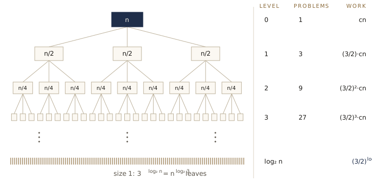
Each call does \(O(n)\) work of its own, splitting and recombining; say at most \(cm\) steps for a subproblem of size \(m\). The total work at depth \(k\) is
\[3^k \cdot c\,\frac{n}{2^k} = \left(\frac{3}{2}\right)^k cn.\]At the root this is \(cn\). At the leaves, \(k = \log_2 n\), it is \(3^{\log_2 n} \cdot c\). The total is a geometric series with ratio \(3/2 > 1\), and an increasing geometric series is at most a constant times its last term (for ratio \(r > 1\), the sum \(1 + r + \dots + r^m\) is below \(\frac{r}{r-1} r^m\)). So the running time is \(O(3^{\log_2 n})\). To put that in a friendlier form, use the identity
\[a^{\log_b n} = n^{\log_b a},\]which holds because both sides have logarithm (base \(b\)) equal to \(\log_b a \cdot \log_b n\). So \(3^{\log_2 n} = n^{\log_2 3} \approx n^{1.585}\), and Karatsuba’s algorithm runs in time \(O(n^{\log_2 3})\).
With four products instead of three, the tree has the same height, but \(4^{\log_2 n} = n^2\) leaves, so the running time is at least \(n^2\). In divide and conquer, the number of subproblems is the branching factor of the recursion tree, and changing it by one can change the exponent of the running time.
Two practical remarks. First, no real implementation recurses down to single bits: a processor multiplies 64-bit words in one instruction, so the recursion should stop when the numbers fit in a word, or somewhat later, where the schoolbook method on the remaining pieces is faster in practice. Second, we can do better still: the last section of this module, on the fast Fourier transform, develops the idea behind the fastest known multiplication algorithms.
Back to Fibonacci
Module 00 left a question open. fib3 computes \(F_n\) with \(O(\log n)\) multiplications of numbers with up to \(O(n)\) bits, and whether that beats the \(O(n^2)\) of fib2 depends on the cost \(M(n)\) of multiplying \(n\)-bit numbers. Exercise 6 of module 00 showed that fib3 takes \(O(M(n))\) time, because the numbers roughly double in length at each squaring and the last multiplication dominates.
With schoolbook multiplication, \(M(n) = O(n^2)\) and fib3 is no better than fib2 asymptotically. With Karatsuba’s algorithm, \(M(n) = O(n^{1.59})\), and fib3 wins. That is what the timing in module 00 showed: CPython multiplies large integers with Karatsuba’s algorithm (switching to it above a size cutoff). You can see the exponent in a timing experiment. If multiplication took time \(n^2\), doubling \(n\) would multiply the time by 4; for \(n^{1.585}\) it multiplies it by \(2^{1.585} \approx 3\).
import time

def time_product(x, y, repeats=3):
    """Best of a few wall-clock timings of x * y, in seconds."""
    best = float("inf")
    for _ in range(repeats):
        start = time.perf_counter()
        x * y
        best = min(best, time.perf_counter() - start)
    return best

random.seed(7)
previous = None
for bits in [250_000, 500_000, 1_000_000, 2_000_000]:
    best = time_product(random.getrandbits(bits), random.getrandbits(bits), repeats=7)
    ratio = f"x{best / previous:.2f}" if previous else ""
    print(f"{bits:>9,} bits: {best * 1000:7.1f} ms  {ratio}")
    previous = best
  250,000 bits:     7.3 ms
  500,000 bits:    21.9 ms  x3.01
1,000,000 bits:    66.6 ms  x3.04
2,000,000 bits:   209.5 ms  x3.14
Your times will differ, but the ratios should hover around 3, not 4.
Recurrence relations
The general pattern
Karatsuba’s algorithm fits a pattern shared by most divide-and-conquer algorithms: to solve a problem of size \(n\), make \(a\) recursive calls on subproblems of size \(n/b\), and spend \(O(n^d)\) time dividing and combining. Its running time satisfies
\[T(n) = a\,T(\lceil n/b \rceil) + O(n^d)\]for constants \(a > 0\), \(b > 1\), \(d \ge 0\). Karatsuba has \(a = 3\), \(b = 2\), \(d = 1\). Instead of drawing a new recursion tree every time, we solve the general recurrence once.
Theorem (master theorem). Suppose \(T(n) = a\,T(\lceil n/b \rceil) + O(n^d)\) for constants \(a > 0\), \(b > 1\), and \(d \ge 0\). Then \(T(n) = O(n^d)\) if \(d > \log_b a\); \(T(n) = O(n^d \log n)\) if \(d = \log_b a\); and \(T(n) = O(n^{\log_b a})\) if \(d < \log_b a\).
The quantity to compare is \(\log_b a\) against \(d\). In words: if the combining work at the top dominates, the answer is the top level’s cost \(n^d\); if the number of leaves \(n^{\log_b a}\) dominates, the answer is the number of leaves; and if they balance, every level costs the same and we pay \(n^d\) once per level.
Proof, by the recursion tree
The idea is the same as for Karatsuba: add up the work level by level, and notice that the per-level totals form a geometric series.
Assume first that \(n\) is a power of \(b\), so the ceilings disappear. (This costs nothing in the bound: for any \(n\) there is a power of \(b\) between \(n\) and \(bn\), and \(T\) is increasing, so rounding \(n\) up to that power changes \(T(n)\) by at most a constant factor when the answer is a polynomial.) Let the non-recursive work on a subproblem of size \(m\) be at most \(cm^d\).
Each level of recursion divides the subproblem size by \(b\), so the tree has depth \(\log_b n\). Each node has \(a\) children, so depth \(k\) has \(a^k\) subproblems of size \(n/b^k\). The work at depth \(k\) is therefore at most
\[a^k \cdot c\left(\frac{n}{b^k}\right)^d = c\,n^d \left(\frac{a}{b^d}\right)^k.\]Summing over \(k = 0, 1, \dots, \log_b n\) gives a geometric series with first term \(cn^d\) and ratio \(r = a/b^d\). There are three cases.
- \(r < 1\), that is, \(d > \log_b a\). The series decreases, and a decreasing geometric series is at most \(\frac{1}{1-r}\) times its first term. Total: \(O(n^d)\).
- \(r = 1\), that is, \(d = \log_b a\). All \(\log_b n + 1\) terms equal \(cn^d\). Total: \(O(n^d \log n)\).
-
\(r > 1\), that is, \(d < \log_b a\). The series increases, and is at most a constant times its last term:
\[c\,n^d \left(\frac{a}{b^d}\right)^{\log_b n} = c\,n^d \cdot \frac{a^{\log_b n}}{\left(b^{\log_b n}\right)^d} = c\,a^{\log_b n} = c\,n^{\log_b a}.\]Total: \(O(n^{\log_b a})\).
The condition \(r < 1\) is \(a < b^d\), which is \(\log_b a < d\) after taking logarithms; the other two conditions translate the same way. This proves the theorem. The same argument with “at least” in place of “at most” shows that the bounds are tight (\(\Theta\)) when the combining work is \(\Theta(n^d)\).
A helper, and a check
The theorem is mechanical enough to code. The helper below returns the \(\Theta\) bound as a string.
import math

def power_of_n(e):
    if math.isclose(e, 0):
        return "1"
    if math.isclose(e, 1):
        return "n"
    return "n^" + format(e, ".4g")

def master(a, b, d):
    """Solution of T(n) = a T(n/b) + Theta(n^d) by the master theorem."""
    crit = math.log(a, b)            # log_b a
    if math.isclose(d, crit):
        return "Θ(" + ("log n" if d == 0 else power_of_n(d) + " log n") + ")"
    if d > crit:
        return "Θ(" + power_of_n(d) + ")"
    return "Θ(" + power_of_n(crit) + ")"

recurrences = [
    ("binary search",            1, 2, 0),
    ("mergesort",                2, 2, 1),
    ("four half-size products",  4, 2, 1),
    ("Karatsuba",                3, 2, 1),
    ("matrices, 8 block products", 8, 2, 2),
    ("Strassen",                 7, 2, 2),
    ("select, perfect pivot",    1, 2, 1),
]
for name, a, b, d in recurrences:
    print(f"{name:>27}:  a={a} b={b} d={d}  ->  {master(a, b, d)}")
              binary search:  a=1 b=2 d=0  ->  Θ(log n)
                  mergesort:  a=2 b=2 d=1  ->  Θ(n log n)
    four half-size products:  a=4 b=2 d=1  ->  Θ(n^2)
                  Karatsuba:  a=3 b=2 d=1  ->  Θ(n^1.585)
 matrices, 8 block products:  a=8 b=2 d=2  ->  Θ(n^3)
                   Strassen:  a=7 b=2 d=2  ->  Θ(n^2.807)
      select, perfect pivot:  a=1 b=2 d=1  ->  Θ(n)
The table is a preview: every line is an algorithm from this module. To check the theorem numerically, compute the recurrence exactly, with \(T(1) = 1\) and combining cost exactly \(n^d\), and divide by the predicted bound. If the theorem is right, the ratio should settle at a constant.
from functools import cache

def exact_T(a, b, d):
    @cache
    def T(n):
        return 1 if n == 1 else a * T(n // b) + n ** d
    return T

cases = [(3, 2, 1, lambda n: n ** math.log2(3)),           # d < log_b a
         (2, 2, 1, lambda n: n * math.log2(n)),            # d = log_b a
         (2, 2, 2, lambda n: n ** 2)]                      # d > log_b a
print(" " * 26 + "n =  " + "  ".join(f"{'2^' + str(k):>6}" for k in [5, 10, 20, 40]))
for a, b, d, bound in cases:
    T = exact_T(a, b, d)
    ratios = "  ".join(f"{T(2 ** k) / bound(2 ** k):6.3f}" for k in [5, 10, 20, 40])
    print(f"a={a} b={b} d={d}:  T(n) / {master(a, b, d)[2:-1]:<8}  {ratios}")
                          n =     2^5    2^10    2^20    2^40
a=3 b=2 d=1:  T(n) / n^1.585    2.737   2.965   2.999   3.000
a=2 b=2 d=1:  T(n) / n log n    1.200   1.100   1.050   1.025
a=2 b=2 d=2:  T(n) / n^2        1.969   1.999   2.000   2.000
The ratios settle at 3, 1, and 2 respectively, as the geometric-series argument predicts: in the first case the leaves contribute \(n^{\log_2 3}\) and the series is at most \(\frac{r}{r-1} = 3\) times its last term; in the second, each of the \(\log_2 n + 1\) levels costs \(n\); in the third, the series \(n^2(1 + \frac12 + \frac14 + \cdots)\) approaches \(2n^2\).
Watch out. The master theorem covers only recurrences of the form \(aT(n/b) + O(n^d)\). It says nothing about \(T(n) = T(n-1) + O(1)\) (subproblems that shrink by subtraction, not division), \(T(n) = 2T(n/2) + O(n \log n)\) (combining cost that is not a pure power of \(n\)), or recursions that split into unequal parts such as \(T(n) = T(n/3) + T(2n/3) + O(n)\). For those, draw the recursion tree or expand the recurrence by hand; exercise 3 has examples.
Binary search
Binary search looks for a key \(k\) in a sorted list \(z[0], \dots, z[n-1]\). Compare \(k\) with the middle element; if it is smaller, the key can only be in the left half, otherwise only in the right half. One comparison halves the problem, so
\[T(n) = T(\lceil n/2 \rceil) + O(1),\]which is \(a = 1\), \(b = 2\), \(d = 0\) in the master theorem: \(d = \log_2 1 = 0\), so \(T(n) = O(\log n)\). It is divide and conquer in its purest form, with a single subproblem and nothing to combine.
def binary_search(z, key):
    """Index of key in the sorted list z, or None if it is absent."""
    lo, hi = 0, len(z)                 # if key is present, it is in z[lo:hi]
    while lo < hi:
        mid = (lo + hi) // 2
        ops["probes"] += 1
        if z[mid] == key:
            return mid
        if z[mid] < key:
            lo = mid + 1
        else:
            hi = mid
    return None

z = list(range(0, 2_000_000, 2))       # one million even numbers
random.seed(3)
worst = 0
for key in random.sample(range(2_000_000), 2000):
    ops.clear()
    i = binary_search(z, key)
    assert (i is not None) == (key % 2 == 0) and (i is None or z[i] == key)
    worst = max(worst, ops["probes"])
print("n =", len(z), "  most probes in 2000 searches:", worst)
print("log2 n =", round(math.log2(len(z)), 2))
n = 1000000   most probes in 2000 searches: 20
log2 n = 19.93
A million elements, and never more than 20 probes. Exercise 5 asks you to prove the matching lower bound: any algorithm that learns about the list only through comparisons needs about \(\log_2 n\) of them.
Mergesort
Split, sort, merge
Sorting has an obvious divide-and-conquer algorithm. Split the list into two halves, sort each half recursively, and merge the two sorted halves into one sorted list. That is mergesort.
Merging is where the work is. Given sorted lists \(x\) and \(y\), the smallest element overall is either \(x[0]\) or \(y[0]\), whichever is smaller. Move it to the output and repeat with what remains. When one list runs out, append the rest of the other. The book writes merge recursively; the loop below does the same thing with two indices, and counts the element comparisons.
def merge(x, y):
    """Merge two sorted lists into one sorted list."""
    z, i, j = [], 0, 0
    while i < len(x) and j < len(y):
        ops["comparisons"] += 1
        if x[i] <= y[j]:
            z.append(x[i])
            i += 1
        else:
            z.append(y[j])
            j += 1
    z.extend(x[i:])                    # at most one of these two
    z.extend(y[j:])                    # is non-empty
    return z

def mergesort(a):
    """Sorted copy of the list a."""
    if len(a) <= 1:
        return list(a)
    mid = len(a) // 2
    return merge(mergesort(a[:mid]), mergesort(a[mid:]))

print(merge([2, 7, 8], [1, 3, 9, 10]))
print(mergesort([9, 4, 7, 1, 12, 3, 8, 5]))

random.seed(4)
lists = [[random.randrange(100) for _ in range(random.randrange(60))]
         for _ in range(500)]
print(all(mergesort(a) == sorted(a) for a in lists))
[1, 2, 3, 7, 8, 9, 10]
[1, 3, 4, 5, 7, 8, 9, 12]
True
Correctness. For merge, the loop keeps this invariant: z holds the \(i + j\) smallest elements of \(x\) and \(y\) combined, in sorted order. It holds at the start, and each iteration appends the smaller of \(x[i]\) and \(y[j]\), which is the smallest element not yet in z because both lists are sorted. When the loop ends, the leftover elements of one list are all at least as large as everything in z. For mergesort, induct on the length: lists of length 0 or 1 are sorted, and if the two recursive calls return sorted halves, merge returns the sorted whole.
Running time. Every comparison in merge moves one element to the output, so merging lists of total length \(m\) takes at most \(m - 1\) comparisons and \(O(m)\) time. Mergesort’s recurrence is
the balanced case of the master theorem (\(d = 1 = \log_2 2\)), so \(T(n) = O(n \log n)\). The recursion tree shows it directly: \(\log_2 n\) levels, and at each level the merges handle \(n\) elements in total.
random.seed(5)
for n in [1_000, 10_000, 100_000]:
    a = [random.random() for _ in range(n)]
    ops.clear()
    mergesort(a)
    print(f"n = {n:>7,}   comparisons = {ops['comparisons']:>9,}"
          f"   n log2 n = {n * math.log2(n):>11,.0f}")
n =   1,000   comparisons =     8,696   n log2 n =       9,966
n =  10,000   comparisons =   120,348   n log2 n =     132,877
n = 100,000   comparisons = 1,536,403   n log2 n =   1,660,964
The comparison counts sit just below \(n \log_2 n\), as the analysis promises.
Mergesort without recursion
All the real work happens in the merges, and they start only when the recursion reaches single elements. From the bottom, the singletons are merged in pairs, the pairs are merged into runs of four, and so on, until one sorted list remains.
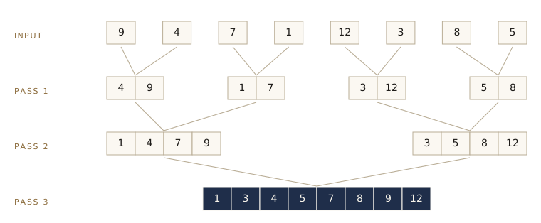
This view gives an iterative algorithm. Keep a queue of sorted lists, initially the \(n\) singletons. Repeatedly remove the two lists at the front, merge them, and add the result at the back. When one list is left, it is the answer. Python’s collections.deque is a queue with constant-time operations at both ends.
from collections import deque

def mergesort_queue(a):
    """Bottom-up mergesort driven by a queue of sorted lists."""
    if not a:
        return []
    Q = deque([x] for x in a)          # n sorted lists of length 1
    while len(Q) > 1:
        Q.append(merge(Q.popleft(), Q.popleft()))
    return Q.popleft()

print(mergesort_queue([9, 4, 7, 1, 12, 3, 8, 5]))
print(all(mergesort_queue(a) == sorted(a) for a in lists))

random.seed(5)
for n in [1_024, 1_000, 100_000]:
    a = [random.random() for _ in range(n)]
    ops.clear(); mergesort(a); rec = ops["comparisons"]
    ops.clear(); mergesort_queue(a); que = ops["comparisons"]
    print(f"n = {n:>7,}   recursive: {rec:>9,}   queue: {que:>9,}")
[1, 3, 4, 5, 7, 8, 9, 12]
True
n =   1,024   recursive:     8,925   queue:     8,925
n =   1,000   recursive:     8,721   queue:     8,716
n = 100,000   recursive: 1,536,625   queue: 1,542,482
When \(n\) is a power of 2, the queue performs exactly the passes of the figure: the \(n/2\) merges of the first pass come off the front before any merged pair does, then the \(n/4\) merges of the second pass, and so on. For other \(n\) the merged lists are slightly less balanced than in the recursive version, but the comparison counts above stay close, and the \(O(n \log n)\) bound still holds.
A lower bound for sorting
Can a cleverer algorithm sort with fewer than about \(n \log_2 n\) comparisons? Not if it learns about the input only by comparing elements. The argument is one of the few proofs in this course that a problem cannot be solved faster, by any algorithm at all.
Any comparison-based sorting algorithm, run on inputs of a fixed size \(n\), can be drawn as a decision tree. Each internal node is a comparison such as “\(a_i < a_j\)?”, with one child for each answer. The algorithm starts at the root, and the outcome of each comparison decides which comparison it makes next. At a leaf it stops, and the leaf records the sorted order it has determined. Here is the tree of insertion sort on three elements \(a_1, a_2, a_3\):
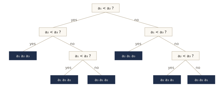
The number of comparisons the algorithm makes on an input is the length of the path from the root to the leaf that input reaches. So the worst-case number of comparisons is the depth of the tree, the length of its longest root-to-leaf path.
Theorem. Every comparison-based sorting algorithm makes \(\Omega(n \log n)\) comparisons on some input of size \(n\).
Proof. Take the decision tree for inputs of size \(n\) with distinct elements. Every one of the \(n!\) orderings must appear at some leaf: if some ordering \(\pi\) were missing, then an input arranged according to \(\pi\) would end at a leaf that reports a different order, and the algorithm would be wrong on it. So the tree has at least \(n!\) leaves. A binary tree of depth \(h\) has at most \(2^h\) leaves (induct on \(h\): each extra level at most doubles the number of leaves). Hence \(2^h \ge n!\), and the depth is
\[h \ge \log_2 (n!).\]Finally, \(\log_2(n!) = \Omega(n \log n)\): at least \(n/2\) of the factors \(1, 2, \dots, n\) are at least \(n/2\), so \(n! \ge (n/2)^{n/2}\) and \(\log_2(n!) \ge \frac{n}{2}\log_2 \frac{n}{2}\). ∎
So mergesort is optimal among comparison sorts, up to a constant factor. For small \(n\) we can compare the exact bound \(\lceil \log_2 n! \rceil\) with mergesort’s actual worst case, by running mergesort on every permutation.
from itertools import permutations

print(" n   ceil(log2 n!)   mergesort worst case")
for n in range(2, 9):
    worst = 0
    for p in permutations(range(n)):
        ops.clear()
        mergesort(list(p))
        worst = max(worst, ops["comparisons"])
    print(f"{n:>2}   {math.ceil(math.log2(math.factorial(n))):>13}   {worst:>20}")
 n   ceil(log2 n!)   mergesort worst case
 2               1                      1
 3               3                      3
 4               5                      5
 5               7                      8
 6              10                     11
 7              13                     14
 8              16                     17
Mergesort is within one comparison of the information-theoretic bound for these sizes. Asymptotically the two differ by a factor that approaches 1: \(\log_2(n!) = n\log_2 n - n\log_2 e + O(\log n)\) by Stirling’s formula, while mergesort makes at most \(n\lceil \log_2 n\rceil\) comparisons.
The fine print matters. The theorem is about algorithms that access the elements only through comparisons. An algorithm that looks at the elements’ values can sometimes do better: integers in a small range \(0, \dots, M\) can be sorted in \(O(n + M)\) time by counting how many times each value occurs, with no comparisons between elements at all (exercise 7). The lower bound does not apply because such an algorithm does not fit the decision-tree model.
Medians and selection
The problem
The median of a list of numbers is the middle value when the list is sorted: half the numbers are at most the median and half are at least it. For an even-length list there are two middle values; we take the smaller one. The median of \([31, 4, 18, 9, 26]\) is 18.
The median, like the mean (average), summarizes a list by one typical value, and it has two advantages: it is always one of the data values, and it is robust to outliers. The list \([5, 6, 5, 7, 6]\) has mean 5.8 and median 6. If one value is mistyped as 7000, the mean jumps above 1000 while the median does not move.
We can find the median by sorting, in \(O(n \log n)\) time. But sorting computes the order of all the elements, and we want only one of them, so we might hope for linear time. To design a recursive algorithm, it helps to solve a more general problem, because the recursion will need it:
Selection. Given a list \(S\) of numbers and an integer \(k\) with \(1 \le k \le \lvert S \rvert\), return the \(k\)th smallest element of \(S\).
With \(k = 1\) this is the minimum; with \(k = \lceil \lvert S \rvert / 2 \rceil\) it is the median.
Splitting around a pivot
Pick any element \(v\) of \(S\), called the pivot, and split \(S\) into three lists: \(S_L\), the elements smaller than \(v\); \(S_v\), the elements equal to \(v\); and \(S_R\), the elements larger than \(v\). For \(S = [14, 3, 22, 8, 14, 30, 1, 17, 5, 11]\) and \(v = 11\):
\[S_L = [3, 8, 1, 5], \qquad S_v = [11], \qquad S_R = [14, 22, 14, 30, 17].\]Comparing \(k\) with the sizes of these lists tells us which one holds the answer. If we want the 7th smallest element, it is not in \(S_L\) or \(S_v\), which hold only the 5 smallest, so it is the 2nd smallest element of \(S_R\). In general,
\[\text{selection}(S, k) = \begin{cases} \text{selection}(S_L, k) & \text{if } k \le \lvert S_L \rvert, \\ v & \text{if } \lvert S_L \rvert < k \le \lvert S_L \rvert + \lvert S_v \rvert, \\ \text{selection}(S_R,\ k - \lvert S_L \rvert - \lvert S_v \rvert) & \text{if } k > \lvert S_L \rvert + \lvert S_v \rvert. \end{cases}\]The split takes one pass over \(S\), so linear time, and then we recurse on one list only. How much that helps depends on the pivot. If it were always the median, each call would halve the list and the running time would be \(T(n) = T(n/2) + O(n) = O(n)\). But the median is what we are trying to find. The way out is surprisingly simple: choose the pivot at random.
def selection(S, k):
    """The k-th smallest element of S (k = 1 is the minimum), with a random pivot."""
    ops["elements scanned"] += len(S)
    v = random.choice(S)
    SL, Sv, SR = [], [], []
    for x in S:                                   # one pass: the split
        if x < v:
            SL.append(x)
        elif x == v:
            Sv.append(x)
        else:
            SR.append(x)
    if k <= len(SL):
        return selection(SL, k)
    if k <= len(SL) + len(Sv):
        return v
    return selection(SR, k - len(SL) - len(Sv))

S = [14, 3, 22, 8, 14, 30, 1, 17, 5, 11]
random.seed(10)
print([selection(S, k) for k in range(1, len(S) + 1)])
print(sorted(S))

ok = True
for trial in range(300):
    # short lists of small numbers, so there are many duplicates
    T = [random.randrange(50) for _ in range(random.randrange(1, 80))]
    k = random.randrange(1, len(T) + 1)
    ok = ok and selection(T, k) == sorted(T)[k - 1]
print(ok)
[1, 3, 5, 8, 11, 14, 14, 17, 22, 30]
[1, 3, 5, 8, 11, 14, 14, 17, 22, 30]
True
Correctness does not depend on the pivot at all: whatever \(v\) is, the three cases above are right, and each recursive call is on a strictly shorter list (it excludes \(v\)), so the recursion ends. Only the running time is random.
Expected running time
In the worst case the pivot is always the largest (or smallest) remaining element, the list shrinks by only one element per call, and finding the median costs \(n + (n-1) + \dots + n/2 = \Theta(n^2)\). That happens with tiny probability. To show the typical cost is linear, call a pivot good if it lies between the 25th and 75th percentiles of the list it was chosen from. A good pivot has at least a quarter of the list on each side, so both \(S_L\) and \(S_R\) have at most \(3/4\) of the elements. Half of the elements of any list are good pivots, so a random pivot is good with probability \(1/2\).
Lemma (waiting for heads). If each trial succeeds independently with probability \(1/2\), the expected number of trials up to and including the first success is 2.
Proof. Let \(E\) be that expected number. We always make one trial; with probability \(1/2\) it fails and we are back where we started, facing an expected \(E\) more trials. So \(E = 1 + \frac12 E\), which gives \(E = 2\). ∎
So on average two splits are enough to shrink the list to at most \(3/4\) of its size, and each split costs \(O(n)\) on a list of size at most \(n\). Let \(T(n)\) be the expected running time on a list of size \(n\). Taking expectations of
\[\text{time on size } n \;\le\; \text{time on size } \tfrac{3}{4}n \;+\; \text{time for the splits that shrink it to } \tfrac34 n,\]and using that the expectation of a sum is the sum of the expectations, we get
\[T(n) \le T(3n/4) + O(n).\]This is the master theorem with \(a = 1\), \(b = 4/3\), \(d = 1\), and \(d > \log_{4/3} 1 = 0\), so \(T(n) = O(n)\). Unrolled, the bound is a geometric series \(cn(1 + \frac34 + \frac{9}{16} + \cdots) \le 4cn\).
Let us measure the constant. The counter adds up the length of every list the algorithm scans, which is proportional to its running time.
random.seed(431)
for n in [1_000, 10_000, 100_000]:
    total = 0
    for trial in range(10):
        S = [random.randrange(10 * n) for _ in range(n)]
        k = (n + 1) // 2                          # the median
        ops.clear()
        assert selection(S, k) == sorted(S)[k - 1]
        total += ops["elements scanned"]
    print(f"n = {n:>7,}   average elements scanned per element: {total / 10 / n:.2f}")
n =   1,000   average elements scanned per element: 3.47
n =  10,000   average elements scanned per element: 3.23
n = 100,000   average elements scanned per element: 3.19
The work per element stays flat, a little under 3.5, as \(n\) grows a hundredfold: linear time, with a small constant.
Notice that the randomness here is in the algorithm, not in the input. The bound holds for every input list, on average over the algorithm’s own coin flips; no input is bad for it, only unlucky runs are, and those are rare. There is also a deterministic linear-time selection algorithm (Blum, Floyd, Pratt, Rivest, and Tarjan, 1973) that chooses the pivot as the median of medians of groups of five, but its constant factor is larger, and in practice the randomized version (or a hybrid of the two) is usually preferred.
Quicksort
Mergesort and selection split in opposite ways. Mergesort splits by position (first half, second half), paying nothing to split and working hard to merge. Selection splits by value (smaller than the pivot, larger than the pivot) and has nothing to combine afterward.
Quicksort sorts by splitting like selection: choose a random pivot, split into \(S_L\), \(S_v\), \(S_R\), sort \(S_L\) and \(S_R\) recursively, and concatenate. Its worst case is \(\Theta(n^2)\), again from persistently bad pivots, but its expected running time is \(O(n \log n)\) (exercise 8), and in practice it is very fast, because the split can be done in place with a tight inner loop. Quicksort and its refinements are the basis of many library sorting routines.
Matrix multiplication
The definition and the obvious algorithm
The product of two \(n \times n\) matrices \(X\) and \(Y\) is the \(n \times n\) matrix \(Z = XY\) with entries
\[Z_{ij} = \sum_{k=1}^{n} X_{ik} Y_{kj},\]the dot product of row \(i\) of \(X\) with column \(j\) of \(Y\). Computing \(n^2\) entries at \(n\) multiplications each gives an \(O(n^3)\) algorithm. (Matrix multiplication is not commutative: in general \(XY \ne YX\).) Matrices are lists of rows here.
def mat_mult_naive(X, Y):
    """Product of two square matrices (lists of rows), straight from the definition."""
    n = len(X)
    Z = [[0] * n for _ in range(n)]
    for i in range(n):
        for j in range(n):
            for k in range(n):
                ops["scalar mults"] += 1
                Z[i][j] += X[i][k] * Y[k][j]
    return Z

X = [[1, 2], [3, 4]]
Y = [[0, 5], [6, 7]]
print(mat_mult_naive(X, Y), mat_mult_naive(Y, X))
[[12, 19], [24, 43]] [[15, 20], [27, 40]]
For a long time \(O(n^3)\) was believed to be optimal, and Strassen’s 1969 algorithm, which beats it with divide and conquer, came as a surprise.
Block multiplication
Matrix multiplication can be done blockwise. Cut \(X\) and \(Y\) (with \(n\) even) into four \(n/2 \times n/2\) blocks each:
\[X = \begin{pmatrix} A & B \\ C & D \end{pmatrix}, \qquad Y = \begin{pmatrix} E & F \\ G & H \end{pmatrix}, \qquad XY = \begin{pmatrix} AE + BG & AF + BH \\ CE + DG & CF + DH \end{pmatrix}.\]The formula is the \(2 \times 2\) product with blocks in place of numbers (exercise 9 asks you to prove it). It gives a divide-and-conquer algorithm with eight half-size products and \(O(n^2)\) work to add blocks:
\[T(n) = 8\,T(n/2) + O(n^2).\]Here \(\log_2 8 = 3 > 2 = d\), so the master theorem gives \(O(n^3)\): no gain, just as with four products for integers.
Strassen’s seven products
As with integers, the improvement comes from algebra that saves one product. Strassen found that seven half-size products suffice:
\[\begin{aligned} P_1 &= A(F - H), & P_5 &= (A + D)(E + H), \\ P_2 &= (A + B)H, & P_6 &= (B - D)(G + H), \\ P_3 &= (C + D)E, & P_7 &= (A - C)(E + F), \\ P_4 &= D(G - E), & & \end{aligned}\] \[XY = \begin{pmatrix} P_5 + P_4 - P_2 + P_6 & P_1 + P_2 \\ P_3 + P_4 & P_1 + P_5 - P_3 - P_7 \end{pmatrix}.\]Check one entry to see how the terms cancel. The top-right block should be \(AF + BH\), and \(P_1 + P_2 = AF - AH + AH + BH = AF + BH\). The top-left block takes more cancelling: \(P_5 + P_4 - P_2 + P_6\) expands to \(AE + AH + DE + DH + DG - DE - AH - BH + BG + BH - DG - DH\), which collapses to \(AE + BG\). Because block multiplication does not commute, every product in these expansions keeps its left factor on the left, and the cancellations never need \(AB = BA\).
def mat_add(X, Y):
    return [[a + b for a, b in zip(r, s)] for r, s in zip(X, Y)]

def mat_sub(X, Y):
    return [[a - b for a, b in zip(r, s)] for r, s in zip(X, Y)]

def quarters(X):
    """The four blocks of X: top-left, top-right, bottom-left, bottom-right."""
    h = len(X) // 2
    return ([r[:h] for r in X[:h]], [r[h:] for r in X[:h]],
            [r[:h] for r in X[h:]], [r[h:] for r in X[h:]])

def from_quarters(TL, TR, BL, BR):
    return [a + b for a, b in zip(TL, TR)] + [a + b for a, b in zip(BL, BR)]

def strassen(X, Y):
    """Product of two n x n matrices, n a power of 2, with seven recursive products."""
    if len(X) == 1:
        ops["scalar mults"] += 1
        return [[X[0][0] * Y[0][0]]]
    A, B, C, D = quarters(X)
    E, F, G, H = quarters(Y)
    P1 = strassen(A, mat_sub(F, H))
    P2 = strassen(mat_add(A, B), H)
    P3 = strassen(mat_add(C, D), E)
    P4 = strassen(D, mat_sub(G, E))
    P5 = strassen(mat_add(A, D), mat_add(E, H))
    P6 = strassen(mat_sub(B, D), mat_add(G, H))
    P7 = strassen(mat_sub(A, C), mat_add(E, F))
    return from_quarters(mat_add(mat_sub(mat_add(P5, P4), P2), P6),
                         mat_add(P1, P2),
                         mat_add(P3, P4),
                         mat_sub(mat_sub(mat_add(P1, P5), P3), P7))

print(strassen(X, Y) == mat_mult_naive(X, Y))

random.seed(6)
print(f"{'n':>3} {'naive mults':>12} {'Strassen mults':>15}  same product?")
for n in [1, 2, 4, 8, 16, 32]:
    X = [[random.randint(-9, 9) for _ in range(n)] for _ in range(n)]
    Y = [[random.randint(-9, 9) for _ in range(n)] for _ in range(n)]
    ops.clear(); Z1 = mat_mult_naive(X, Y); naive = ops["scalar mults"]
    ops.clear(); Z2 = strassen(X, Y); fast = ops["scalar mults"]
    print(f"{n:>3} {naive:>12,} {fast:>15,}  {Z1 == Z2}")
True
  n  naive mults  Strassen mults  same product?
  1            1               1  True
  2            8               7  True
  4           64              49  True
  8          512             343  True
 16        4,096           2,401  True
 32       32,768          16,807  True
The naive count is \(n^3 = 8^{\log_2 n}\); Strassen’s is exactly \(7^{\log_2 n} = n^{\log_2 7}\). The recurrence is
\[T(n) = 7\,T(n/2) + O(n^2),\]and since \(\log_2 7 \approx 2.807 > 2\), the master theorem gives \(T(n) = O(n^{\log_2 7}) \approx O(n^{2.81})\).
What to notice. Strassen’s algorithm does 18 block additions and subtractions per call instead of 4, so its constant factor is larger, and practical implementations switch to the ordinary method below a few hundred rows. It also needs padding when \(n\) is not a power of 2, and in floating point it is somewhat less numerically stable than the direct method. Since 1969, algorithms with smaller exponents have been found (the best known today is below 2.38), but they are of theoretical interest only; whether \(n^{2 + \epsilon}\) is achievable for every \(\epsilon > 0\) is an open problem.
The fast Fourier transform
Multiplying polynomials
Our last problem is multiplying polynomials. If \(A(x) = a_0 + a_1 x + \dots + a_d x^d\) and \(B(x) = b_0 + b_1 x + \dots + b_d x^d\), their product \(C(x) = A(x)B(x)\) has degree \(2d\) and coefficients
\[c_k = a_0 b_k + a_1 b_{k-1} + \dots + a_k b_0 = \sum_{i=0}^{k} a_i b_{k-i},\]taking \(a_i = b_i = 0\) for \(i > d\). For example, \((2 + x + 3x^2)(1 + 4x + x^2) = 2 + 9x + 9x^2 + 13x^3 + 3x^4\). Computing all \(2d + 1\) coefficients this way takes \(\Theta(d^2)\) arithmetic operations. We represent a polynomial by its list of coefficients, lowest degree first.
def poly_mult_naive(A, B):
    """Coefficients of A(x) * B(x); lists hold coefficients from x^0 upward."""
    C = [0] * (len(A) + len(B) - 1)
    for i, a in enumerate(A):
        for j, b in enumerate(B):
            ops["coefficient mults"] += 1
            C[i + j] += a * b
    return C

poly_mult_naive([2, 1, 3], [1, 4, 1])
[2, 9, 9, 13, 3]
Note. The formula for \(c_k\) is called a convolution, and it is everywhere. Polynomials and integers are close cousins: the digits of a number are the coefficients of a polynomial evaluated at \(x = 10\) (or 2), and multiplying numbers is convolving their digits and then propagating carries. In signal processing, a system that is linear and time-invariant (a filter, an echo, a blur) is described completely by its response \(b\) to a single impulse; its response to any sampled signal \(a\) is the convolution of \(a\) with \(b\). Fast convolution is fast filtering, which is why the algorithm below changed signal processing.
The algorithm we develop, the fast Fourier transform (FFT), multiplies polynomials in \(O(n \log n)\) operations. It takes a few steps to build, and each step is a small idea.
Two ways to describe a polynomial
Fact. A polynomial of degree at most \(d\) is determined by its values at any \(d + 1\) distinct points. (Two points determine a line; three determine a parabola.) We prove this below using linear algebra.
So a polynomial \(A(x)\) of degree at most \(d\) has two representations, once we fix distinct points \(x_0, \dots, x_d\):
- its coefficient representation \(a_0, a_1, \dots, a_d\);
- its value representation \(A(x_0), A(x_1), \dots, A(x_d)\).
Multiplication is easy in the value representation. The product \(C = AB\) has degree \(2d\), so it is determined by its values at \(2d + 1\) points, and its value at any point \(z\) is \(C(z) = A(z) B(z)\): one multiplication per point, linear time in all. The inputs and output are coefficients, though, so we need to convert. That suggests the following plan, for polynomials \(A\) and \(B\) of degree at most \(d\):
- Selection. Choose \(n \ge 2d + 1\) distinct points \(x_0, \dots, x_{n-1}\).
- Evaluation. Compute \(A(x_j)\) and \(B(x_j)\) for every \(j\).
- Multiplication. Compute \(C(x_j) = A(x_j)B(x_j)\) for every \(j\).
- Interpolation. Recover the coefficients of \(C\) from its values.
Steps 1 and 3 take linear time. Evaluating a polynomial at one point takes \(O(n)\) operations (Horner’s rule, in the code below), so evaluating at \(n\) points in the obvious way takes \(\Theta(n^2)\), and interpolation looks even harder. The FFT does both in \(O(n \log n)\), for a well-chosen set of points.
Evaluation by divide and conquer
Suppose we choose the points in plus–minus pairs: \(\pm x_0, \pm x_1, \dots, \pm x_{n/2-1}\). Then the work for \(A(x_j)\) and \(A(-x_j)\) overlaps, because even powers of \(x_j\) and \(-x_j\) are equal. To exploit this, split \(A\) into its even-numbered and odd-numbered coefficients. For instance,
\[5 + 2x + x^2 - 3x^3 + 4x^4 + 7x^5 = (5 + x^2 + 4x^4) + x\,(2 - 3x^2 + 7x^4).\]Both parenthesized pieces are polynomials in \(x^2\). In general
\[A(x) = A_e(x^2) + x\,A_o(x^2),\]where \(A_e\) has the even-numbered coefficients and \(A_o\) the odd-numbered ones; in the example \(A_e(z) = 5 + z + 4z^2\) and \(A_o(z) = 2 - 3z + 7z^2\). If \(A\) has degree at most \(n - 1\), then \(A_e\) and \(A_o\) have degree at most \(n/2 - 1\). Now the pair \(\pm x_j\) costs little more than one point:
\[A(x_j) = A_e(x_j^2) + x_j A_o(x_j^2), \qquad A(-x_j) = A_e(x_j^2) - x_j A_o(x_j^2).\]Evaluating \(A\) at \(n\) paired points reduces to evaluating two polynomials of half the degree, \(A_e\) and \(A_o\), at the \(n/2\) points \(x_0^2, \dots, x_{n/2-1}^2\), plus \(O(n)\) work. If we could keep recursing, the running time would be \(T(n) = 2T(n/2) + O(n) = O(n \log n)\).
The catch is the next level. The new points \(x_j^2\) must themselves be plus–minus pairs, and squares of real numbers are never negative. We need numbers whose squares can be negative: complex numbers.
The complex roots of unity
A complex number \(z = a + bi\) is a point \((a, b)\) in the plane. In polar form it is \(z = r(\cos\theta + i \sin\theta) = re^{i\theta}\), where \(r = \sqrt{a^2 + b^2}\) is its length and \(\theta\) its angle from the positive real axis. Polar form makes multiplication easy: multiply the lengths and add the angles,
\[r_1 e^{i\theta_1} \cdot r_2 e^{i\theta_2} = r_1 r_2\, e^{i(\theta_1 + \theta_2)}.\]In particular, \(-1 = e^{i\pi}\), so negating a number adds \(\pi\) to its angle, and a number of length 1 raised to the power \(n\) has its angle multiplied by \(n\).
Work backward from the bottom of the recursion, where we evaluate at a single point; take it to be 1. The level above needs a plus–minus pair whose squares are 1: that is \(\pm 1\). The level above that needs square roots of \(+1\) and \(-1\): that is \(\pm 1\) and \(\pm i\). Continuing, the \(n\) points at the top are the complex \(n\)th roots of unity, the \(n\) solutions of \(z^n = 1\):
\[1, \omega, \omega^2, \dots, \omega^{n-1}, \qquad \text{where } \omega = e^{2\pi i/n}.\]They are equally spaced around the unit circle, at angles that are multiples of \(2\pi/n\). We call \(\omega\) a primitive \(n\)th root of unity because its powers run through all \(n\) roots before repeating; \(\omega^{-1} = e^{-2\pi i/n}\) is primitive too, while \(\omega^2\) is not (its powers repeat after \(n/2\) steps).
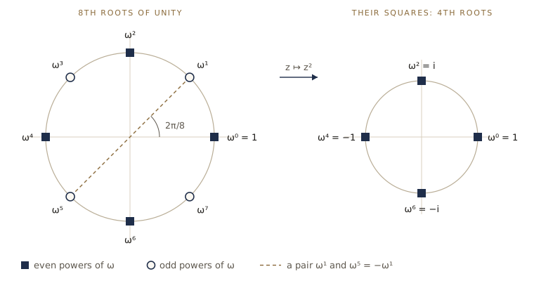
For \(n\) even, the roots have the two properties the recursion needs:
- They are plus–minus paired: \(\omega^{n/2} = e^{i\pi} = -1\), so \(\omega^{j + n/2} = -\omega^j\).
- Their squares are the \((n/2)\)th roots of unity: \((\omega^j)^2 = (\omega^2)^j\), and \(\omega^2 = e^{2\pi i/(n/2)}\) generates the \((n/2)\)th roots. Each of those appears twice among the squares, since \(\omega^j\) and \(\omega^{j+n/2}\) have the same square.
So if \(n\) is a power of 2, then at depth \(k\) of the recursion the points are the \((n/2^k)\)th roots of unity, which are again paired, all the way down to the single point 1.
The FFT algorithm
Put the pieces together. To evaluate \(A\) (degree at most \(n - 1\), \(n\) a power of 2) at \(\omega^0, \omega^1, \dots, \omega^{n-1}\), recursively evaluate \(A_e\) and \(A_o\) at the powers of \(\omega^2\), obtaining \(s_j = A_e(\omega^{2j})\) and \(s'_j = A_o(\omega^{2j})\) for \(j = 0, \dots, n/2 - 1\). Then, for each such \(j\),
\[A(\omega^j) = s_j + \omega^j s'_j, \qquad A(\omega^{j + n/2}) = s_j - \omega^j s'_j.\]The second line uses both properties: \(\omega^{j+n/2} = -\omega^j\), and \((\omega^{j+n/2})^2 = \omega^{2j}\).
import cmath

def fft(a, omega):
    """Values of the polynomial with coefficients a at omega^0, ..., omega^(n-1).

    n = len(a) must be a power of 2, and omega a primitive n-th root of unity.
    """
    n = len(a)
    if n == 1:
        return list(a)                        # a constant polynomial: its value is a[0]
    s = fft(a[0::2], omega * omega)           # A_e at the (n/2)-th roots of unity
    s_odd = fft(a[1::2], omega * omega)       # A_o at the (n/2)-th roots of unity
    r = [0] * n
    w = 1                                     # w = omega^j
    for j in range(n // 2):
        ops["complex mults"] += 1
        t = w * s_odd[j]
        r[j] = s[j] + t
        r[j + n // 2] = s[j] - t
        w *= omega
    return r

fft([1, 2, 3, 4], 1j)       # A(x) = 1 + 2x + 3x^2 + 4x^3 at 1, i, -1, -i
[10, (-2-2j), -2, (-2+2j)]
Check by hand: \(A(1) = 10\), \(A(i) = 1 + 2i - 3 - 4i = -2 - 2i\), \(A(-1) = 1 - 2 + 3 - 4 = -2\), and \(A(-i) = 1 - 2i - 3 + 4i = -2 + 2i\). (With \(\omega = i\) every value is computed exactly; with a general \(\omega\) the entries carry small floating-point errors.) Next, compare with direct evaluation by Horner’s rule, \(a_0 + x(a_1 + x(a_2 + \cdots))\), on a larger random polynomial.
def evaluate(a, x):
    """Horner's rule: the value at x of the polynomial with coefficients a."""
    value = 0
    for c in reversed(a):
        value = value * x + c
    return value

random.seed(8)
n = 64
a = [random.randint(-5, 5) for _ in range(n)]
omega = cmath.exp(2j * cmath.pi / n)
values = fft(a, omega)
error = max(abs(values[j] - evaluate(a, omega ** j)) for j in range(n))
print(f"largest difference from Horner's rule: {error:.1e}")
largest difference from Horner's rule: 4.5e-12
The two agree to within \(10^{-11}\). The running time satisfies \(T(n) = 2T(n/2) + O(n)\), since each call does two half-size calls and a loop of \(n/2\) iterations, so the FFT runs in \(O(n \log n)\) time: \(\frac{n}{2}\log_2 n\) multiplications by powers of \(\omega\), against \(n^2\) for Horner’s rule at every point.
Interpolation, and the matrix view
We can now go from coefficients to values in \(O(n \log n)\). For the last step of the plan we need to go back. The cleanest way to see how is to write evaluation as a matrix–vector product. For points \(x_0, \dots, x_{n-1}\),
\[\begin{pmatrix} A(x_0) \\ A(x_1) \\ \vdots \\ A(x_{n-1}) \end{pmatrix} = \begin{pmatrix} 1 & x_0 & x_0^2 & \cdots & x_0^{n-1} \\ 1 & x_1 & x_1^2 & \cdots & x_1^{n-1} \\ \vdots & & & & \vdots \\ 1 & x_{n-1} & x_{n-1}^2 & \cdots & x_{n-1}^{n-1} \end{pmatrix} \begin{pmatrix} a_0 \\ a_1 \\ \vdots \\ a_{n-1} \end{pmatrix}.\]The matrix in the middle, call it \(M\), is a Vandermonde matrix, and a standard fact of linear algebra is that it is invertible when the \(x_j\) are distinct. That proves the fact we assumed earlier: the values at \(n\) distinct points determine the \(n\) coefficients, namely \(a = M^{-1} \cdot (\text{values})\). So
- evaluation is multiplication by \(M\), and
- interpolation is multiplication by \(M^{-1}\).
When the points are the powers of \(\omega\), the matrix is \(M_n(\omega)\), whose entry in row \(j\), column \(k\) (counting from 0) is \(\omega^{jk}\). The FFT is a fast way to multiply a vector by \(M_n(\omega)\). Its inverse turns out to be almost the same matrix. To see why, recall that two vectors \(u, v\) of complex numbers are orthogonal when their inner product \(\sum_l u_l \overline{v_l}\) is zero; the bar denotes complex conjugation, \(\overline{a + bi} = a - bi\).
Lemma. Let \(\omega = e^{2\pi i/n}\) and \(0 \le j, k < n\). The inner product of columns \(j\) and \(k\) of \(M_n(\omega)\), namely \(\sum_{l=0}^{n-1} \omega^{lj}\, \overline{\omega^{lk}}\), equals \(n\) if \(j = k\) and \(0\) if \(j \ne k\). In other words, the columns are orthogonal.
Proof. A number on the unit circle has conjugate equal to its inverse, so \(\overline{\omega^{lk}} = \omega^{-lk}\) and the sum is \(\sum_{l} \omega^{l(j-k)}\). If \(j = k\), every term is 1 and the sum is \(n\). Otherwise \(q = \omega^{j-k} \ne 1\) (since \(0 < \lvert j - k \rvert < n\)), and the sum is the geometric series \(1 + q + \dots + q^{n-1} = \frac{1 - q^n}{1 - q} = 0\), because \(q^n = (\omega^n)^{j-k} = 1\). ∎
In matrix form, the lemma says \(\overline{M}^{\,T} M = nI\), where \(\overline{M}^{\,T}\) is the conjugate transpose. Since \(M_n(\omega)\) is symmetric and its conjugate has entries \(\omega^{-jk}\), the conjugate transpose is \(M_n(\omega^{-1})\). This gives the inversion formula
\[M_n(\omega)^{-1} = \frac{1}{n} M_n(\omega^{-1}).\]And \(\omega^{-1}\) is also a primitive \(n\)th root of unity (it goes around the circle the other way), so multiplying by \(M_n(\omega^{-1})\) is again an FFT. Interpolation is the FFT run with \(\omega^{-1}\) in place of \(\omega\), followed by division by \(n\):
\[\text{values} = \mathrm{FFT}(\text{coefficients}, \omega), \qquad \text{coefficients} = \frac{1}{n}\,\mathrm{FFT}(\text{values}, \omega^{-1}).\]Geometrically, the orthogonal columns of \(M_n(\omega)\) form a new coordinate system, the Fourier basis, and the FFT is a change of basis into it (a rotation, up to the scale factor \(\sqrt{n}\)). The inverse FFT rotates back. Polynomial multiplication is hard in the standard basis (coefficients) and easy in the Fourier basis (values), so we rotate, multiply, and rotate back.
Multiplying polynomials with the FFT
All four steps of the plan are now in place. Pad both coefficient lists with zeros to length \(n\), the first power of 2 that is at least the number of coefficients of the product; the points are the \(n\)th roots of unity.
def inverse_fft(values, omega):
    n = len(values)
    return [v / n for v in fft(values, 1 / omega)]   # 1/omega is omega^(-1)

def poly_mult_fft(A, B):
    """Coefficients of A(x) * B(x) for integer coefficients, via the FFT."""
    m = len(A) + len(B) - 1                  # number of coefficients of the product
    n = 1
    while n < m:
        n *= 2
    omega = cmath.exp(2j * cmath.pi / n)
    values_A = fft(A + [0] * (n - len(A)), omega)                  # evaluation
    values_B = fft(B + [0] * (n - len(B)), omega)
    values_C = [x * y for x, y in zip(values_A, values_B)]         # multiplication
    C = inverse_fft(values_C, omega)                               # interpolation
    return [round(c.real) for c in C[:m]]

print(poly_mult_fft([2, 1, 3], [1, 4, 1]))

random.seed(9)
ok = True
for trial in range(200):
    A = [random.randint(-100, 100) for _ in range(random.randint(1, 70))]
    B = [random.randint(-100, 100) for _ in range(random.randint(1, 70))]
    ok = ok and poly_mult_fft(A, B) == poly_mult_naive(A, B)
print(ok)
[2, 9, 9, 13, 3]
True
The products agree with the naive method on 200 random pairs. Here is what the interpolation step returns for the small example before poly_mult_fft rounds it:
n = 8
omega = cmath.exp(2j * cmath.pi / n)
values = [x * y for x, y in zip(fft([2, 1, 3] + [0] * 5, omega),
                                fft([1, 4, 1] + [0] * 5, omega))]
for c in inverse_fft(values, omega)[:5]:
    print(c)
(1.9999999999999993+8.881784197001252e-16j)
(9+0j)
(9-9.43689570931383e-16j)
(13-8.881784197001252e-16j)
(3.000000000000001+0j)
The true coefficients are 2, 9, 9, 13, 3. The tiny imaginary parts and the digits far after the decimal point are floating-point noise, and rounding the real part recovers the exact integers. Now compare operation counts: the naive method multiplies every coefficient of \(A\) with every coefficient of \(B\), while the FFT method runs three FFTs of size \(n\) plus \(n\) pointwise products.
random.seed(11)
print(f"{'degree':>7} {'naive mults':>12} {'FFT mults':>10}")
for d in [15, 63, 255, 1023, 4095]:
    A = [random.randint(0, 9) for _ in range(d + 1)]
    B = [random.randint(0, 9) for _ in range(d + 1)]
    ops.clear()
    C = poly_mult_fft(A, B)
    n = 1 << (2 * d).bit_length()          # the FFT size used above
    fft_mults = ops["complex mults"] + n   # butterflies + pointwise products
    naive = (d + 1) ** 2
    if d <= 255:
        assert C == poly_mult_naive(A, B)
    print(f"{d:>7,} {naive:>12,} {fft_mults:>10,}")
 degree  naive mults  FFT mults
     15          256        272
     63        4,096      1,472
    255       65,536      7,424
  1,023    1,048,576     35,840
  4,095   16,777,216    167,936
For degree 4095, about 16.8 million multiplications shrink to about 168 thousand (complex ones, each worth a few real multiplications). Each time the degree grows by a factor of 4, the naive count grows by 16, while the FFT count grows by about 5 and that factor is falling toward 4, as \(n \log n\) predicts.
Watch out. The FFT here works in floating point, and rounding is only safe while the accumulated error stays below 0.5. For very long polynomials with large coefficients (for example, when multiplying integers with millions of digits), the errors can grow past that. Serious implementations either bound the coefficient size carefully or do the whole computation in modular arithmetic, with a root of unity modulo a prime in place of \(\omega\); the algebra above goes through unchanged, and there is no rounding at all. Exercise 11 explores this.
The FFT unrolled: butterflies
Look at one step of the FFT from outside. Each pair of outputs \((r_j, r_{j+n/2})\) is computed from the pair \((s_j, s'_j)\) by multiplying \(s'_j\) by \(\omega^j\) once and then adding and subtracting. Drawn as a circuit, with wires carrying complex numbers, the two inputs cross over to the two outputs in a shape called a butterfly. Unrolling the whole recursion gives a circuit of \(\log_2 n\) stages, each a column of \(n/2\) butterflies.
In which order do the coefficients enter the first stage? The top-level call sends the even-indexed coefficients to one half and the odd-indexed to the other; the next level splits each half again by the next bit of the index, and so on. So the leaves are ordered by the last bit of the index, then the second-to-last bit, and so on: the order is bit reversal.
def leaf_order(indices):
    """The order in which the FFT recursion reaches the coefficients."""
    if len(indices) == 1:
        return indices
    return leaf_order(indices[0::2]) + leaf_order(indices[1::2])

def bit_reverse(j, bits):
    return int(format(j, "0" + str(bits) + "b")[::-1], 2)

print(leaf_order(list(range(8))))
print([bit_reverse(j, 3) for j in range(8)])
print([format(j, "03b") for j in leaf_order(list(range(8)))])
[0, 4, 2, 6, 1, 5, 3, 7]
[0, 4, 2, 6, 1, 5, 3, 7]
['000', '100', '010', '110', '001', '101', '011', '111']
The coefficient in position \(j\) of the first stage is \(a_{\text{rev}(j)}\): position 1 holds \(a_4\) because \(001\) reversed is \(100\). This observation gives the iterative FFT: permute the input into bit-reversed order, then run \(\log_2 n\) passes of butterflies over the array, in place, with no recursion (exercise 10). The circuit also explains why the FFT suits hardware and parallel machines: every butterfly in a stage is independent of the others, so an entire stage can be computed at once.
Where the FFT leads
Two remarks close the chapter. First, integers: an \(n\)-bit number is a polynomial in \(x = 2\) (or in \(x = 2^{w}\), using \(w\)-bit blocks as coefficients), so an FFT-based polynomial product plus carry propagation multiplies integers. Refining this idea, Schönhage and Strassen (1971) multiplied \(n\)-bit integers in \(O(n \log n \log\log n)\) time, and Harvey and van der Hoeven (2021) reached \(O(n \log n)\). These methods pay off only for very large numbers, and the libraries that do arbitrary-precision arithmetic switch among schoolbook, Karatsuba-style, and FFT-based multiplication as the numbers grow.
Second, history. Cooley and Tukey published the FFT in 1965, and it spread quickly, first through signal processing and then everywhere. The idea itself is older: it appears in unpublished work of Gauss from the early 1800s, which brings the chapter back to where it started.
Summary
| Problem | Algorithm | Recurrence | Running time |
|---|---|---|---|
| multiply two \(n\)-bit integers | Karatsuba (three half-size products) | \(T(n) = 3T(n/2) + O(n)\) | \(O(n^{\log_2 3}) \approx O(n^{1.59})\) |
| search a sorted list | binary search | \(T(n) = T(n/2) + O(1)\) | \(O(\log n)\) |
| sort \(n\) elements | mergesort (recursive or with a queue) | \(T(n) = 2T(n/2) + O(n)\) | \(O(n \log n)\), optimal for comparison sorts |
| \(k\)th smallest of \(n\) | randomized selection | \(T(n) \le T(3n/4) + O(n)\) in expectation | \(O(n)\) expected, \(\Theta(n^2)\) worst case |
| multiply two \(n \times n\) matrices | Strassen (seven half-size products) | \(T(n) = 7T(n/2) + O(n^2)\) | \(O(n^{\log_2 7}) \approx O(n^{2.81})\) |
| multiply two degree-\(d\) polynomials | FFT, pointwise product, inverse FFT | \(T(n) = 2T(n/2) + O(n)\) per FFT | \(O(n \log n)\) with \(n \approx 2d\) |
The master theorem, for \(T(n) = aT(n/b) + O(n^d)\):
| Condition | Which levels dominate | Solution |
|---|---|---|
| \(d > \log_b a\) | the root | \(O(n^d)\) |
| \(d = \log_b a\) | all levels equally | \(O(n^d \log n)\) |
| \(d < \log_b a\) | the leaves | \(O(n^{\log_b a})\) |
Ideas to carry forward:
- The number of subproblems is the branching factor of the recursion tree. Saving one subproblem (four to three, eight to seven) lowers the exponent, because the saving compounds at every level.
- To analyze a divide-and-conquer algorithm, sum the work level by level; the level totals form a geometric series, and the largest term wins.
- Lower bounds are possible: counting the leaves of a decision tree shows that no comparison sort beats \(\Omega(n \log n)\).
- A good representation can make a hard operation easy. Polynomials multiply pointwise in the value representation, and the FFT converts between representations in \(O(n \log n)\) time.
Exercises
- Multiply \(x = 10110011_2\) and \(y = 01101101_2\) by hand with Karatsuba’s algorithm, recursing down to 2-bit numbers. List the three products at the top level and check your answer against
karatsuba. - Show that the recurrence \(T(n) = 3T(\lceil n/2 \rceil + 1) + cn\) still has solution \(O(n^{\log_2 3})\). (Hint: substitute \(S(n) = T(n + 2)\), or show directly that the subproblem sizes at depth \(k\) are at most \(n/2^k + 2\).)
- Solve each recurrence with a \(\Theta\) bound, using the master theorem where it applies and a recursion tree or expansion where it does not: (a) \(T(n) = 2T(n/4) + 1\); (b) \(T(n) = 6T(n/3) + n^2\); (c) \(T(n) = 16T(n/4) + n^2\); (d) \(T(n) = 3T(n/3) + n^{1.5}\); (e) \(T(n) = T(n - 1) + n\); (f) \(T(n) = 2T(n - 1) + 1\); (g) \(T(n) = 2T(n/2) + n \log n\); (h) \(T(n) = T(\sqrt{n}) + 1\).
- Algorithm P solves a problem of size \(n\) by solving six subproblems of size \(n/3\) and combining in \(O(n)\) time. Algorithm Q solves three subproblems of size \(n - 1\) and combines in \(O(1)\). Algorithm R solves four subproblems of size \(n/2\) and combines in \(O(n^2)\). Give each running time and say which you would use.
- Prove that any algorithm that searches a sorted list of \(n\) elements using only comparisons of the form “is \(z[i] \le k\)?” must make at least \(\lceil \log_2(n+1) \rceil\) comparisons in the worst case. (Hint: a decision tree again; how many different answers must it be able to give?)
- Write a function that merges \(k\) sorted lists of \(n\) elements each. First merge them one at a time into a growing result and find its running time in terms of \(k\) and \(n\). Then merge them in pairs, divide-and-conquer style, and show that this takes \(O(nk \log k)\) time. Count comparisons in both versions for \(k = 64\), \(n = 100\).
- Implement counting sort for a list of integers in the range \(0, \dots, M\) and show it runs in \(O(n + M)\) time. Explain precisely which step of the \(\Omega(n \log n)\) proof fails for it.
- (a) Write quicksort using the three-way split of
selectionand a random pivot, and check it againstsorted(). (b) Show that its worst case is \(\Theta(n^2)\). (c) For a list of \(n\) distinct elements, count \(n - 1\) comparisons for a split. Show that the expected number of comparisons \(Q(n)\) satisfies \(Q(n) \le n - 1 + \frac{1}{n}\sum_{i=0}^{n-1}\left(Q(i) + Q(n-1-i)\right)\), and prove \(Q(n) \le 2n \ln n\) for \(n \ge 1\) by induction (bound the sum by an integral). (d) Compare the average comparison count with mergesort’s for \(n = 10^4\). - Prove the block multiplication formula: if \(X\) and \(Y\) are split into \(n/2 \times n/2\) blocks \(A, \dots, H\) as in the notes, the top-left block of \(XY\) is \(AE + BG\), and similarly for the other three blocks. Then verify by expanding all four entries that Strassen’s formulas are correct.
- Write an iterative FFT: permute the coefficients into bit-reversed order, then run \(\log_2 n\) passes of butterflies in place over one list. Check it against
ffton random inputs of length 1024 and confirm that it performs the same number of complex multiplications. - Modular FFT. (a) Show that \(3\) has order 16 modulo 17, so \(\omega = 3\) plays the role of a primitive 16th root of unity in arithmetic mod 17. (b) Adapt
fftto integers mod 17 (replace1 / omegaby the inverse of \(\omega\) mod 17, and \(1/n\) by the inverse of \(n\) mod 17) and use it, with the coefficients padded to length 16, to multiply \(1 + 2x + 3x^2\) by \(4 + 5x\), checking the coefficients mod 17. (c) Why can a modular FFT never suffer from rounding error? - In your own words: explain to a classmate why Karatsuba’s “save one multiplication out of four” lowers the exponent of the running time, while saving one addition out of four in the combine step would not change the exponent at all. Use the recursion tree in your explanation.
Going further
- Dasgupta, Papadimitriou, and Vazirani, Algorithms, chapter 2 — the source for this module. Exercises 2.3–2.5 practice recurrences, 2.15 does the split in place, 2.23 finds majority elements, 2.24 analyzes quicksort, 2.27 shows that squaring matrices is as hard as multiplying them, and 2.32 develops a divide-and-conquer algorithm for the closest pair of points.
- Volker Strassen, “Gaussian elimination is not optimal”, Numerische Mathematik, 1969 — the three-page paper with the seven products.
- James W. Cooley and John W. Tukey, “An algorithm for the machine calculation of complex Fourier series”, Mathematics of Computation, 1965 — the paper that made the FFT widely known.
- Manuel Blum, Robert Floyd, Vaughan Pratt, Ronald Rivest, and Robert Tarjan, “Time bounds for selection”, Journal of Computer and System Sciences, 1973 — deterministic linear-time selection with the median of medians.
- Karatsuba algorithm and Fast Fourier transform on Wikipedia — worked examples, variants, and pointers to how real libraries choose among multiplication algorithms.
These notes follow the chapters of S. Dasgupta, C. H. Papadimitriou, and U. V. Vazirani, Algorithms (McGraw-Hill, 2008), the course text. The explanations, code, figures, and exercises here are written for this course; the book remains the reference, with many more exercises.