CSE 431/531 · Module 01 · Weeks 1–2
Algorithms with Numbers
Arithmetic on n-bit numbers, modular arithmetic, primality testing, RSA, and universal hashing.
Companion reading: Dasgupta, Papadimitriou & Vazirani, Algorithms, chapter 1, “Algorithms with numbers”
By the end of this module you can
- Measure the size of a number in bits and analyze addition, multiplication, and division by counting bit operations.
- Compute modulo \(N\) with the substitution rule, and raise numbers to huge powers modulo \(N\) by repeated squaring.
- Run Euclid’s algorithm and its extension by hand, prove them correct, and show that they take a polynomial number of steps.
- Decide when a number has a multiplicative inverse modulo \(N\), and compute it.
- Prove Fermat’s little theorem, explain why the randomized Fermat test errs with probability at most \(1/2\) per round, and name the numbers that defeat it.
- Generate a random \(n\)-bit prime in expected polynomial time, using the prime number theorem.
- Explain how RSA encrypts and decrypts, prove that decryption undoes encryption, and say what its security rests on.
- Define a universal family of hash functions, prove that the family built from a prime and a random vector is universal, and use it to bound the expected cost of a hash-table lookup.
Contents
- Numbers and their size
- Addition
- Multiplication
- Division
- Modular arithmetic
- Euclid’s algorithm for the greatest common divisor
- Primality testing
- Cryptography
- Universal hashing
- Summary
- Exercises
- Going further
Two problems about whole numbers look almost the same. Factoring: given a number \(N\), write it as a product of primes. Primality: given a number \(N\), decide whether it is prime. Each seems to need the other: to know that 91 is not prime, you would naturally find its factors 7 and 13. Yet the two problems are worlds apart. The best known factoring methods take time that grows faster than any polynomial in the number of digits of \(N\), while primality can be decided in polynomial time. This module builds the tools that show why, and then puts the gap to work: the RSA cryptosystem is secure precisely because one of the two problems is easy and the other, as far as anyone knows, is hard.
In module 00 we found that the Fibonacci numbers grow so fast that adding two of them cannot count as a single step, and we promised that adding two \(k\)-bit numbers takes time proportional to \(k\). We start by keeping that promise. We then analyze multiplication and division, move to arithmetic modulo \(N\), and build from there, one algorithm at a time, to primality testing, cryptography, and hashing. Along the way we meet our first randomized algorithms, algorithms that flip coins and are still reliable.
Throughout the module, \(n\) is the number of bits of the numbers involved. All running times are counted in bit operations — steps that touch a constant number of bits — because the numbers we care about, a few thousand bits long, are far too large for one machine instruction.
Numbers and their size
Bases and logs
A number is written in base \(b\) as a string of digits from \(\{0, 1, \dots, b-1\}\), the rightmost digit counting ones, the next counting \(b\)’s, the next \(b^2\)’s, and so on. With \(k\) digits we can write every number from \(0\) to \(b^k - 1\) and no more (three decimal digits reach 999). So the number of digits needed for \(N \ge 0\) is the smallest \(k\) with \(b^k > N\):
\[k = \lceil \log_b (N + 1) \rceil \approx \log_b N .\]Changing the base changes the length by a constant factor, since \(\log_b N = \log_a N / \log_a b\). A number has about \(\log_2 10 \approx 3.32\) times as many binary digits as decimal ones. In big-O terms the base does not matter, so we say that \(N\) has size \(O(\log N)\), and when we write \(\log\) without a base we mean \(\log_2\).
We store numbers as lists of bits, least significant bit first, so that position \(i\) of the list holds the coefficient of \(2^i\). That makes “drop the last bit” and “add a zero at the end” into list operations, which is all our arithmetic needs.
import math

def to_bits(x):
    """Binary digits of x >= 0, least significant first; 0 is the empty list."""
    bits = []
    while x > 0:
        bits.append(x % 2)
        x //= 2
    return bits

def from_bits(bits):
    """The number a list of bits stands for (inverse of to_bits)."""
    return sum(b * 2 ** i for i, b in enumerate(bits))

def show(bits):
    """Bits written the usual way, most significant first."""
    return "".join(str(b) for b in reversed(bits)) or "0"

print(to_bits(45), "->", show(to_bits(45)), "->", from_bits(to_bits(45)))
for N in [45, 1_000, 10 ** 100]:
    binary, decimal = len(to_bits(N)), len(str(N))
    predicted = math.ceil(math.log2(N + 1))
    print(f"{decimal:>3} decimal digits, {binary:>3} bits "
          f"(ceil(log2(N+1)) = {predicted}), ratio {binary / decimal:.2f}")
[1, 0, 1, 1, 0, 1] -> 101101 -> 45
  2 decimal digits,   6 bits (ceil(log2(N+1)) = 6), ratio 3.00
  4 decimal digits,  10 bits (ceil(log2(N+1)) = 10), ratio 2.50
101 decimal digits, 333 bits (ceil(log2(N+1)) = 333), ratio 3.30
The ratio approaches \(3.32\) as the numbers grow. The function \(\log N\) will turn up again and again in this course, in several guises that are worth recognizing:
- It is the power to which 2 must be raised to give \(N\).
- It is the number of times you can halve \(N\) before reaching 1 (exactly \(\lfloor \log N \rfloor\) times if you round down after each halving), so an algorithm that halves a number at each step runs for about \(\log N\) steps.
- It is (again up to rounding, \(\lceil \log (N+1) \rceil\)) the number of bits of \(N\).
- It is the depth of a complete binary tree with \(N\) nodes (\(\lfloor \log N \rfloor\), exactly).
- It is, within a constant factor, the harmonic sum \(1 + \tfrac12 + \tfrac13 + \dots + \tfrac1N\) (exercise 1).
Items 2 and 3 are the same fact seen twice: halving a number is dropping its last bit.
Addition
Grade-school addition rests on one small fact: three single digits add up to at most two digits. In decimal, \(9 + 9 + 9 = 27\); in binary, \(1 + 1 + 1 = 3 = 11_2\). So if we add two numbers column by column from the right, the carry into each column is a single digit, each column adds three single digits, and the result of each column is one digit of the answer plus a one-digit carry. Here is \(45 + 27 = 72\) in binary:
\[\begin{array}{rccccccc} \text{carry} & 1 & 1 & 1 & 1 & 1 & 1 & \\ & & 1 & 0 & 1 & 1 & 0 & 1 \\ + & & 0 & 1 & 1 & 0 & 1 & 1 \\ \hline & 1 & 0 & 0 & 1 & 0 & 0 & 0 \end{array}\]The code follows the same steps. It counts one bit operation for each column: combining three bits into a sum bit and a carry bit is work of constant size, whatever the base.
bit_ops = 0          # one per column: three bits in, a sum bit and a carry bit out

def add(x, y):
    """x + y for bit lists, by the grade-school carry method."""
    global bit_ops
    result, carry = [], 0
    for i in range(max(len(x), len(y))):
        xi = x[i] if i < len(x) else 0
        yi = y[i] if i < len(y) else 0
        s = xi + yi + carry          # at most 3, so two bits
        result.append(s % 2)
        carry = s // 2
        bit_ops += 1
    if carry:
        result.append(carry)
    return result

total = add(to_bits(45), to_bits(27))
print(show(total), "=", from_bits(total), "  columns:", bit_ops)
1001000 = 72 columns: 6
To trust the code on large inputs, we compare it with Python’s own addition on random numbers of several sizes, and record the count.
import random
random.seed(1)

def random_nbit(n):
    """A random number with exactly n bits."""
    return random.randrange(2 ** (n - 1), 2 ** n)

for n in [8, 64, 512, 4096]:
    x, y = random_nbit(n), random_nbit(n)
    bit_ops = 0
    ok = from_bits(add(to_bits(x), to_bits(y))) == x + y
    print(f"n = {n:4d}   correct: {ok}   bit operations: {bit_ops}")
n =    8   correct: True   bit operations: 8
n =   64   correct: True   bit operations: 64
n =  512   correct: True   bit operations: 512
n = 4096   correct: True   bit operations: 4096
Correctness. Column \(i\) receives the carry from column \(i-1\), and the invariant “the columns processed so far, plus the pending carry times \(2^i\), equal the sum of the low \(i\) bits of \(x\) and \(y\)” holds after every column; at the end it says the result is \(x + y\).
Running time. Two \(n\)-bit numbers take exactly \(n\) column steps, plus constant overhead, so addition takes \(O(n)\) time. Can we do better? No: any algorithm must at least read the \(2n\) input bits and write the \(n+1\) output bits. Addition is optimal up to a constant factor.
Note. A processor adds two 64-bit numbers in one instruction, so why count bits? Two reasons. The numbers in cryptography have thousands of bits, and arithmetic on them is done word by word, in loops much like
add. And even the one-instruction adder is a circuit whose size grows with the number of bits. Counting bit operations — the bit complexity — accounts for both.
Multiplication
The grade-school method in binary
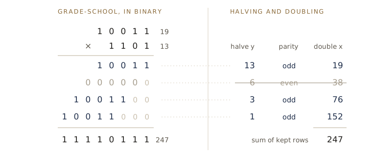
To multiply \(x\) by \(y\) in grade school you multiply \(x\) by each digit of \(y\), shift each partial product left by the digit’s position, and add the rows. In binary each row is either \(0\) or a shifted copy of \(x\), and shifting left by one position multiplies by 2. The left half of the figure multiplies \(19 = 10011_2\) by \(13 = 1101_2\).
There is an older way to do the same multiplication without writing \(y\) in binary. Put the two numbers side by side, then repeatedly halve the left one (rounding down) and double the right one, until the left reaches 1. Cross out the rows where the left number is even, and add up what remains on the right. It looks unrelated, but it is the binary method in disguise: the parity of the halved numbers spells out the bits of \(y\), from the last bit up, and the doubled numbers are exactly the shifted copies of \(x\).
def shift(x, k):
    """x times 2**k, for a bit list x: put k zeros in front of the lowest bit."""
    return [0] * k + x if x else []

def multiply_school(x, y):
    """x * y for bit lists: add a shifted copy of x for every 1 bit of y."""
    total = []
    for i, bit in enumerate(y):
        if bit == 1:
            total = add(total, shift(x, i))
    return total

product = multiply_school(to_bits(19), to_bits(13))
print(show(product), "=", from_bits(product))
11110111 = 247
Why it is correct: writing \(y = \sum_i y_i 2^i\) with bits \(y_i\), distributivity gives \(xy = \sum_i y_i \,(x \cdot 2^i)\), and the loop adds exactly those terms. For the running time, there are at most \(n\) rows, each at most \(2n\) bits long, and each addition costs \(O(n)\), so the total is \(O(n) \cdot n = O(n^2)\). Multiplication is quadratic, where addition was linear.
The halving rule as a recursive algorithm
The halving-and-doubling method becomes a short recursive algorithm if we write it as a rule about \(x \cdot y\). Let \(\lfloor y/2 \rfloor\) be \(y\) halved and rounded down (in binary: drop the last bit). Then
\[x \cdot y = \begin{cases} 2\,(x \cdot \lfloor y/2 \rfloor) & \text{if } y \text{ is even}, \\ x + 2\,(x \cdot \lfloor y/2 \rfloor) & \text{if } y \text{ is odd}. \end{cases}\]The rule is true because \(y = 2\lfloor y/2 \rfloor\) when \(y\) is even and \(y = 2\lfloor y/2 \rfloor + 1\) when \(y\) is odd; multiply both sides by \(x\). In the code, every operation is on bit lists: halving is y[1:], the parity is y[0], doubling is shift(z, 1).
def multiply(x, y):
    """x * y for bit lists, by the halving rule."""
    if not y:                        # y = 0
        return []
    z = multiply(x, y[1:])           # y[1:] is floor(y / 2)
    if y[0] == 0:                    # y even: 2z
        return shift(z, 1)
    return add(x, shift(z, 1))       # y odd: x + 2z

random.seed(2)
print("small products correct:",
      all(from_bits(multiply(to_bits(a), to_bits(b))) == a * b
          for a in range(64) for b in range(64)))
for n in [32, 64, 128, 256, 512]:
    bit_ops = 0
    for _ in range(10):                          # ten random pairs of n-bit numbers
        x, y = random_nbit(n), random_nbit(n)
        assert from_bits(multiply(to_bits(x), to_bits(y))) == x * y
    avg = bit_ops / 10
    print(f"n = {n:3d}   average bit operations {avg:9,.0f}",
          f"  per n^2 {avg / n**2:.3f}")
small products correct: True
n =  32   average bit operations       775   per n^2 0.756
n =  64   average bit operations     3,343   per n^2 0.816
n = 128   average bit operations    12,772   per n^2 0.780
n = 256   average bit operations    50,540   per n^2 0.771
n = 512   average bit operations   196,222   per n^2 0.749
Correctness is induction on \(y\): the base case \(y = 0\) returns 0, and if the recursive call returns \(x \lfloor y/2 \rfloor\) correctly, the code applies the rule above. Running time: each call removes one bit of \(y\), so there are \(n\) recursive calls. Each does a constant number of shifts, one parity test, and at most one addition, all on numbers of at most \(2n\) bits, for \(O(n)\) bit operations per call and \(O(n^2)\) in total. The counts confirm it: doubling \(n\) multiplies the work by about 4, and the ratio to \(n^2\) stays between about \(0.75\) and \(0.82\). (Only additions are counted; the shifts and parity tests would add another \(O(n)\) per call, which does not change the picture.)
Can we do better? It seems that any method must add up to \(n\) copies of \(x\), each costing \(O(n)\). That intuition is wrong: module 02 multiplies \(n\)-bit numbers in \(O(n^{1.59})\) time by divide and conquer.
Division
To divide an integer \(x \ge 0\) by an integer \(y \ge 1\) is to find the quotient \(q\) and remainder \(r\) with \(x = qy + r\) and \(0 \le r < y\). Division fits the same halving pattern as multiplication: first divide \(\lfloor x/2 \rfloor\) by \(y\), then double the answer and correct it.
def divide(x, y):
    """(q, r) with x = q*y + r and 0 <= r < y, for integers x >= 0 and y >= 1."""
    if x == 0:
        return 0, 0
    q, r = divide(x // 2, y)         # floor(x/2) = q*y + r
    q, r = 2 * q, 2 * r              # so 2*floor(x/2) = q*y + r
    if x % 2 == 1:
        r = r + 1                    # now x = q*y + r, with 0 <= r <= 2y - 1
    if r >= y:
        r, q = r - y, q + 1          # one subtraction brings r below y
    return q, r

print(divide(247, 19), divmod(247, 19))
random.seed(3)
tests = [(random_nbit(300), random_nbit(random.randint(1, 300)))
         for _ in range(1000)]
print("random tests agree with divmod:",
      all(divide(x, y) == divmod(x, y) for x, y in tests))
(13, 0) (13, 0)
random tests agree with divmod: True
Correctness, by induction on \(x\). Suppose the recursive call returns \(q', r'\) with \(\lfloor x/2 \rfloor = q'y + r'\) and \(0 \le r' < y\). Since \(x = 2\lfloor x/2 \rfloor + (x \bmod 2)\), we get \(x = (2q')y + (2r' + x \bmod 2)\), and the new remainder \(2r' + x \bmod 2\) is at most \(2(y-1) + 1 = 2y - 1\). One subtraction of \(y\), if needed, puts it in the range \(0 \le r < y\) while keeping \(x = qy + r\). Running time: there are \(n\) calls (one per bit of \(x\)), each doing a comparison, a subtraction, and some shifts on \(O(n)\)-bit numbers, so division takes \(O(n^2)\) bit operations, like multiplication.
Modular arithmetic
Repeated multiplication makes numbers enormous. Clocks and calendars avoid this by wrapping around: after hour 23 comes hour 0, after day 6 of the week comes day 0. Modular arithmetic does the same for integers in general, and it is the setting for everything from here to the end of the module.
For a positive integer \(N\), \(x \bmod N\) is the remainder of \(x\) divided by \(N\): if \(x = qN + r\) with \(0 \le r < N\), then \(x \bmod N = r\). Two integers are congruent modulo \(N\) if they differ by a multiple of \(N\):
\[x \equiv y \pmod N \iff N \mid (x - y).\](Read \(N \mid m\) as “\(N\) divides \(m\)”.) For example \(100 \equiv 2 \pmod 7\), because \(98 = 14 \cdot 7\): if today is day 2 of the week, then 100 days from day 0 is also day 2. Negative numbers are fine too: \(-1 \equiv 6 \pmod 7\), since yesterday relative to day 0 is day 6.
There are two useful pictures. In the first, arithmetic modulo \(N\) lives on the numbers \(0, 1, \dots, N-1\) arranged in a circle, and anything that leaves the range wraps around. In the second, all integers are allowed, but they are sorted into \(N\) congruence classes \(\{i + kN : k \text{ an integer}\}\), one for each \(i\) from \(0\) to \(N - 1\). Modulo 4, for instance, \(\{\dots, -7, -3, 1, 5, 9, \dots\}\) is one class. Any member of a class can stand in for any other, because of this rule:
Lemma (substitution rule). If \(x \equiv x' \pmod N\) and \(y \equiv y' \pmod N\), then \(x + y \equiv x' + y' \pmod N\) and \(xy \equiv x'y' \pmod N\).
To see it, write \(x' = x + sN\) and \(y' = y + tN\). Then \(x' + y' = (x + y) + (s + t)N\) and \(x'y' = xy + (xt + ys + stN)N\), and both differ from the original by a multiple of \(N\).
The familiar laws — associativity, commutativity, distributivity — hold modulo \(N\) as well, since they hold for the integers and congruence respects \(+\) and \(\times\). Together with the substitution rule, this gives us the working principle of the whole module: in any computation made of additions and multiplications, we may reduce intermediate results modulo \(N\) at any point, and the final answer modulo \(N\) does not change. It can turn an impossible computation into a mental one. What is \(3^{200} \bmod 13\)? Notice that \(3^3 = 27 \equiv 1 \pmod{13}\). Then
\[3^{200} = \left(3^{3}\right)^{66} \cdot 3^{2} \equiv 1^{66} \cdot 9 = 9 \pmod{13}.\]print(3 ** 200 % 13, pow(3, 200, 13))
print(len(str(3 ** 200)), "decimal digits in 3**200")
print((-1) % 7, 100 % 7)
9 9
96 decimal digits in 3**200
6 2
Watch out. Python’s
%always returns a result in \(\{0, \dots, N-1\}\) for positive \(N\), so(-1) % 7is 6. In C, C++, and Java,-1 % 7is \(-1\): the sign follows the dividend. Both are correct representatives of the same congruence class, but code that indexes an array byx % Nbreaks on negativexin those languages.
Note. Two’s complement, the way computers store signed integers, is modular arithmetic. With \(w\) bits, the numbers from \(-2^{w-1}\) to \(2^{w-1} - 1\) are stored modulo \(2^w\), so \(-x\) is stored as \(2^w - x\). Addition and subtraction then work unchanged: add the stored values and discard any overflow bit, which is reduction modulo \(2^w\). For 8 bits, \(-5\) is stored as \(251\), and \(251 + 10 = 261 \equiv 5 \pmod{256}\), which is \(-5 + 10\).
Modular addition and multiplication
Let \(n = \lceil \log N \rceil\) be the number of bits of \(N\), and keep all values in the range \(0\) to \(N - 1\).
- Addition. \(x + y\) is at most \(2(N-1)\); if it is \(N\) or more, subtract \(N\) once. One addition and at most one subtraction of \((n+1)\)-bit numbers: \(O(n)\).
- Multiplication. \(xy\) is at most \((N-1)^2\), which has at most \(2n\) bits. Multiply in \(O(n^2)\), then reduce with one division by \(N\), also \(O(n^2)\). Total: \(O(n^2)\).
- Division is subtler. Modulo \(N\), dividing by \(a\) is possible only for some \(a\), and we come back to it after Euclid’s algorithm. When it is possible, it takes \(O(n^3)\).
Modular exponentiation
RSA needs \(x^y \bmod N\) for numbers \(x\), \(y\), \(N\) that are hundreds or thousands of bits long. Computing \(x^y\) first and reducing at the end is out of the question: \(x^y\) has about \(y \log x\) bits, and for a 1000-bit \(y\) that is more bits than there are atoms in the universe. The substitution rule lets us reduce after every multiplication, so every intermediate result stays below \(N\). But the obvious loop, multiply by \(x\) and reduce, \(y - 1\) times, is still exponential: \(y - 1\) is about \(2^{n}\) multiplications.
The fix is repeated squaring, the same idea that computed Fibonacci numbers with \(O(\log n)\) matrix products in module 00. Squaring \(k\) times reaches \(x^{2^k}\) with only \(k\) multiplications, and any power is a product of such squares, one for each 1 bit of the exponent. For instance \(44 = 101100_2\), so \(x^{44} = x^{32} \cdot x^{8} \cdot x^{4}\). The recursive version of this idea is the rule
\[x^y = \begin{cases} \left(x^{\lfloor y/2 \rfloor}\right)^2 & \text{if } y \text{ is even}, \\ x \cdot \left(x^{\lfloor y/2 \rfloor}\right)^2 & \text{if } y \text{ is odd}, \end{cases}\]applied modulo \(N\). Compare it with the multiplication rule: where multiplication doubles and adds, exponentiation squares and multiplies. The code counts modular multiplications.
mults = 0      # modular multiplications performed

def modexp(x, y, N):
    """x**y mod N, by repeated squaring."""
    global mults
    if y == 0:
        return 1 % N
    z = modexp(x, y // 2, N)
    mults += 1
    if y % 2 == 0:
        return z * z % N
    mults += 1
    return x * (z * z % N) % N

mults = 0
print(modexp(3, 44, 101), pow(3, 44, 101), "  multiplications:", mults)

random.seed(4)
x, y, N = random_nbit(512), random_nbit(512), random_nbit(512)
mults = 0
print("512-bit numbers agree with pow:", modexp(x, y, N) == pow(x, y, N),
      "  multiplications:", mults)
78 78   multiplications: 9
512-bit numbers agree with pow: True   multiplications: 750
For \(y = 44\) the recursion visits \(44, 22, 11, 5, 2, 1\), squaring at each of the six levels and multiplying by \(x\) at the three odd ones: 9 multiplications. A 512-bit exponent takes 750 — compared with the roughly \(2^{511}\) of the obvious loop.
Correctness is induction on \(y\) using the rule above, reduced modulo \(N\) by the substitution rule. Running time. Each call halves \(y\), so there are at most \(n\) calls when \(y\) has \(n\) bits, and each call does one or two multiplications of numbers below \(N\), each followed by a reduction: \(O(n^2)\) per call. With \(x\), \(y\), and \(N\) all \(n\)-bit numbers, modular exponentiation takes \(O(n^3)\) time. Python’s three-argument pow(x, y, N) runs the same repeated-squaring idea (with some refinements) in C; from now on we use it, having checked it against modexp.
Euclid’s algorithm for the greatest common divisor
The greatest common divisor \(\gcd(a, b)\) of two integers is the largest integer that divides both. The obvious approach is to factor both numbers and multiply the common prime factors: \(1716 = 2^2 \cdot 3 \cdot 11 \cdot 13\) and \(1386 = 2 \cdot 3^2 \cdot 7 \cdot 11\), so \(\gcd(1716, 1386) = 2 \cdot 3 \cdot 11 = 66\). But that needs factoring, the problem we believe to be hard. Euclid’s algorithm, more than two thousand years old, avoids it entirely.
Lemma (Euclid’s rule). If \(x \ge y > 0\) are integers, then \(\gcd(x, y) = \gcd(x \bmod y,\ y)\).
The pairs \((x, y)\) and \((x - y, y)\) have exactly the same common divisors: a number dividing \(x\) and \(y\) divides their difference, and a number dividing \(x - y\) and \(y\) divides their sum \(x\). So \(\gcd(x, y) = \gcd(x - y, y)\). Subtracting \(y\) repeatedly, as long as the first argument stays at least \(y\), turns \(x\) into \(x \bmod y\) without changing the gcd.
The rule gives a recursive algorithm directly. Each call swaps the arguments so that the larger comes first.
def euclid(a, b):
    """gcd(a, b) for integers a >= b >= 0."""
    if b == 0:
        return a
    return euclid(b, a % b)

print(euclid(1716, 1386), math.gcd(1716, 1386))
random.seed(5)
pairs = [(random.getrandbits(200), random.getrandbits(200)) for _ in range(2000)]
print("agrees with math.gcd:",
      all(euclid(max(a, b), min(a, b)) == math.gcd(a, b) for a, b in pairs))
66 66
agrees with math.gcd: True
On the example, the calls are \((1716, 1386) \to (1386, 330) \to (330, 66) \to (66, 0)\), which returns 66. Correctness follows from Euclid’s rule and \(\gcd(a, 0) = a\). The running time depends on how fast the arguments shrink, and they shrink fast.
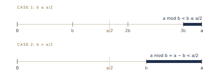
Lemma. If \(a \ge b > 0\), then \(a \bmod b < a/2\).
There are two cases, pictured below. If \(b \le a/2\), then \(a \bmod b < b \le a/2\), because a remainder is always less than the divisor. If \(b > a/2\), then \(b\) fits into \(a\) only once, so \(a \bmod b = a - b < a - a/2 = a/2\).
Running time. One call turns \((a, b)\) into \((b, a \bmod b)\), and the next into \((a \bmod b, \dots)\). By the lemma, after two calls the first argument has dropped from \(a\) to less than \(a/2\): it has lost at least one bit. If \(a\) and \(b\) have \(n\) bits, the base case is reached within \(2n\) calls. Each call does one division, \(O(n^2)\), so Euclid’s algorithm runs in \(O(n^3)\) time.
How close to \(2n\) calls can it get? The worst inputs turn out to be consecutive Fibonacci numbers, which shrink as slowly as possible: \(F_{k+1} \bmod F_k = F_{k-1}\), so the algorithm walks down the whole sequence one step at a time. Here are the step counts for those and for random pairs:
def euclid_steps(a, b):
    """Number of recursive calls euclid(a, b) makes (same algorithm, as a loop)."""
    steps = 0
    while b > 0:
        a, b = b, a % b
        steps += 1
    return steps

fib = [0, 1]
while len(fib) < 1002:
    fib.append(fib[-1] + fib[-2])

for k in [10, 100, 1000]:
    a, b = fib[k + 1], fib[k]
    n = a.bit_length()
    label = f"F({k + 1}), F({k})"
    calls = euclid_steps(a, b)
    print(f"{label:>16}:  n = {n:3d} bits,  calls {calls:4d},  2n = {2 * n}")

random.seed(6)
for n in [100, 1000]:
    pairs = [sorted((random_nbit(n), random_nbit(n)), reverse=True)
             for _ in range(500)]
    avg = sum(euclid_steps(a, b) for a, b in pairs) / len(pairs)
    label = f"random {n}-bit"
    print(f"{label:>16}:  average calls {avg:.0f},  2n = {2 * n}")
    F(11), F(10):  n =   7 bits,  calls    9,  2n = 14
  F(101), F(100):  n =  69 bits,  calls   99,  2n = 138
F(1001), F(1000):  n = 694 bits,  calls  999,  2n = 1388
  random 100-bit:  average calls 59,  2n = 200
 random 1000-bit:  average calls 583,  2n = 2000
For Fibonacci inputs the count is about \(1.44n\) calls, since \(F_k\) has about \(0.694k\) bits; random inputs need only about \(0.58n\). The bound \(2n\) is not tight, but it is the right order: the number of calls is \(\Theta(n)\) in the worst case.
Extended Euclid: a certificate for the gcd
Suppose someone tells you that \(d = \gcd(a, b)\). Checking that \(d\) divides \(a\) and \(b\) shows only that \(d\) is a common divisor, not the greatest one. The following lemma gives a check that proves it is the greatest.
Lemma. If \(d\) divides both \(a\) and \(b\), and \(d = ax + by\) for some integers \(x\) and \(y\), then \(d = \gcd(a, b)\).
Since \(d\) is a common divisor, \(d \le \gcd(a, b)\). Since \(\gcd(a, b)\) divides \(a\) and \(b\), it divides \(ax + by = d\), so \(\gcd(a, b) \le d\). Together, they are equal.
For example, \(\gcd(47, 17) = 1\) because \(47 \cdot 4 + 17 \cdot (-11) = 188 - 187 = 1\). Such coefficients always exist, and a small extension of Euclid’s algorithm finds them along with the gcd.
def extended_euclid(a, b):
    """(x, y, d) with d = gcd(a, b) = a*x + b*y, for integers a >= b >= 0."""
    if b == 0:
        return 1, 0, a
    x1, y1, d = extended_euclid(b, a % b)      # d = b*x1 + (a mod b)*y1
    return y1, x1 - (a // b) * y1, d

x, y, d = extended_euclid(47, 17)
print((x, y, d), "check:", 47 * x + 17 * y)

random.seed(7)
ok = True
for _ in range(2000):
    a, b = sorted((random.getrandbits(300), random.getrandbits(300)), reverse=True)
    x, y, d = extended_euclid(a, b)
    ok = ok and d == math.gcd(a, b) and a * x + b * y == d
print("random 300-bit pairs:", ok)
(4, -11, 1) check: 1
random 300-bit pairs: True
Lemma. For integers \(a \ge b \ge 0\),
extended_euclid(a, b)returns \((x, y, d)\) with \(d = \gcd(a, b) = ax + by\).
Ignoring \(x\) and \(y\), the algorithm is euclid, so \(d = \gcd(a, b)\). For the coefficients we use induction on \(b\). When \(b = 0\), \(a \cdot 1 + 0 \cdot 0 = a = d\). When \(b > 0\), the recursive call is on \((b, a \bmod b)\) with \(a \bmod b < b\), so by the induction hypothesis it returns \(x', y'\) with \(d = bx' + (a \bmod b)\,y'\). Substituting \(a \bmod b = a - \lfloor a/b \rfloor b\) and regrouping:
which is exactly the pair the algorithm returns. The running time is that of Euclid’s algorithm plus \(O(n^2)\) work per call for the new coefficients, which stay at most \(n\) bits long: \(O(n^3)\) in all.
By hand, you run Euclid forward and then substitute backward. For \((47, 17)\):
\[47 = 2 \cdot 17 + 13, \qquad 17 = 1 \cdot 13 + 4, \qquad 13 = 3 \cdot 4 + 1, \qquad 4 = 4 \cdot 1 + 0 .\]Starting from the last nonzero remainder and replacing one remainder at a time:
\[1 = 13 - 3 \cdot 4 = 13 - 3\,(17 - 13) = 4 \cdot 13 - 3 \cdot 17 = 4\,(47 - 2 \cdot 17) - 3 \cdot 17 = 4 \cdot 47 - 11 \cdot 17 .\]Modular division
In ordinary arithmetic, dividing by \(a \ne 0\) is multiplying by \(1/a\). Modular arithmetic has the same idea. We say \(x\) is a multiplicative inverse of \(a\) modulo \(N\) if \(ax \equiv 1 \pmod N\). An inverse, when it exists, is unique modulo \(N\) (exercise 5), and we write it \(a^{-1}\).
Not every nonzero number has one. Modulo 10, no multiple of 4 is congruent to 1: \(4x - 10k\) is always even. The same argument works in general. Any number of the form \(ax + kN\) is a multiple of \(\gcd(a, N)\), so if \(\gcd(a, N) > 1\), then \(ax \bmod N\) is never 1. Conversely, if \(\gcd(a, N) = 1\) — we say \(a\) and \(N\) are relatively prime — then extended Euclid gives integers \(x, y\) with \(ax + Ny = 1\), and reducing modulo \(N\) gives \(ax \equiv 1 \pmod N\).
Theorem (modular division). A number \(a\) has a multiplicative inverse modulo \(N\) if and only if \(\gcd(a, N) = 1\). When the inverse exists, extended Euclid finds it in \(O(n^3)\) time, where \(n\) is the number of bits of \(N\).
From the calculation above, \(4 \cdot 47 - 11 \cdot 17 = 1\), so \(-11 \cdot 17 \equiv 1 \pmod{47}\) and the inverse of 17 modulo 47 is \(-11 \equiv 36\). Check: \(17 \cdot 36 = 612 = 13 \cdot 47 + 1\).
def inverse(a, N):
    """The inverse of a modulo N, if gcd(a, N) = 1."""
    x, y, d = extended_euclid(N, a % N)          # N*x + (a mod N)*y = d
    if d != 1:
        raise ValueError(f"{a} has no inverse modulo {N} (gcd is {d})")
    return y % N

print(inverse(17, 47), pow(17, -1, 47), 17 * inverse(17, 47) % 47)
try:
    inverse(4, 10)
except ValueError as err:
    print(err)

random.seed(8)
N = random_nbit(1024)
candidates = [random.randrange(1, N) for _ in range(300)]
units = [a for a in candidates if math.gcd(a, N) == 1]
print("1024-bit modulus, agrees with pow(a, -1, N):",
      all(inverse(a, N) == pow(a, -1, N) for a in units), f"({len(units)} values)")
36 36 1
4 has no inverse modulo 10 (gcd is 2)
1024-bit modulus, agrees with pow(a, -1, N): True (95 values)
So modulo \(N\) we can divide by exactly the numbers relatively prime to \(N\), and to divide we multiply by the inverse. When \(N\) is a prime \(p\), every \(a\) from 1 to \(p - 1\) is relatively prime to \(p\), so every nonzero number can be divided by. That fact drives the next two sections.
Primality testing
Why trial division does not scale
The obvious primality test tries to divide \(N\) by \(2, 3, 4, \dots\). You may stop at \(\sqrt N\): if \(N = KL\) with \(1 < K \le L\), then \(K \le \sqrt N\). That is a big saving, but not big enough. For an \(n\)-bit number, \(\sqrt N \approx 2^{n/2}\), which is still exponential in \(n\).
def is_prime_trial(N):
    """Primality by trial division; also returns the number of divisions tried."""
    if N < 2:
        return False, 0
    tries, d = 0, 2
    while d * d <= N:
        tries += 1
        if N % d == 0:
            return False, tries
        d += 1
    return True, tries

for n in [20, 30, 40]:
    N = 2 ** (n - 1) + 1
    while not is_prime_trial(N)[0]:
        N += 2
    print(f"{n}-bit prime {N:>14,}:  {is_prime_trial(N)[1]:>9,} divisions")
20-bit prime        524,309:        723 divisions
30-bit prime    536,870,923:     23,169 divisions
40-bit prime 549,755,813,911:    741,454 divisions
Every 10 bits multiply the work by about \(2^{5} = 32\). A 1024-bit prime would need about \(2^{511}\) divisions. Trial division is a factoring method in disguise, and factoring is exactly what we cannot do fast. We need a test that can tell \(N\) is composite without finding a factor.
Fermat’s little theorem
Theorem (Fermat’s little theorem). If \(p\) is prime, then \(a^{p-1} \equiv 1 \pmod p\) for every \(a\) with \(1 \le a < p\).
The idea of the proof: multiplying the nonzero numbers modulo \(p\) by \(a\) only shuffles them. The figure shows the shuffle for \(a = 4\) and \(p = 11\).
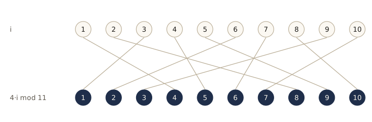
Proof. Let \(S = \{1, 2, \dots, p-1\}\). The numbers \(a \cdot i \bmod p\) for \(i \in S\) are nonzero, since \(p\) is prime and divides neither \(a\) nor \(i\). They are distinct: if \(ai \equiv aj \pmod p\), multiply both sides by \(a^{-1}\) (which exists because \(\gcd(a, p) = 1\)) to get \(i \equiv j\). So they are \(p - 1\) distinct elements of \(S\), which means they are all of \(S\), in some order. Multiply all the elements of \(S\) together in both orders:
\[(p-1)! \equiv \prod_{i=1}^{p-1} (a \cdot i) = a^{p-1} \cdot (p-1)! \pmod p .\]Every factor of \((p-1)!\) is relatively prime to \(p\), so \((p-1)!\) has an inverse modulo \(p\); multiplying both sides by it leaves \(1 \equiv a^{p-1} \pmod p\). \(\square\)
The Fermat test
Fermat’s theorem gives a test that never looks for a factor: pick some \(a\) and compute \(a^{N-1} \bmod N\) by repeated squaring. If the result is not 1, then \(N\) is certainly composite, since a prime would have given 1. If the result is 1, the test says “probably prime”.
The trouble is the second answer. The theorem says what primes do; it does not promise that composites behave differently. Some do not, for some \(a\). Take \(N = 91 = 7 \cdot 13\):
print(pow(2, 90, 91), pow(3, 90, 91))
passing = [a for a in range(1, 91) if pow(a, 90, 91) == 1]
print(len(passing), "of the 90 bases pass for N = 91:", passing[:8], "...")
64 1
36 of the 90 bases pass for N = 91: [1, 3, 4, 9, 10, 12, 16, 17] ...
Base 2 exposes 91, but base 3 is fooled. So we should not fix \(a\) in advance; we should pick it at random and hope that, for a composite \(N\), most bases expose it. For 91, 54 of the 90 bases do. The next lemma says that this is typical, with one exception.
Definition. A Carmichael number is a composite \(N\) with \(a^{N-1} \equiv 1 \pmod N\) for every \(a\) relatively prime to \(N\).
The smallest is \(561 = 3 \cdot 11 \cdot 17\). Carmichael numbers exist in infinite supply, but they are very rare; we set them aside for now and deal with them below.
Lemma. If \(a^{N-1} \not\equiv 1 \pmod N\) for some \(a\) relatively prime to \(N\), then \(a^{N-1} \not\equiv 1 \pmod N\) for at least half of the numbers \(a\) in \(\{1, 2, \dots, N-1\}\).
Proof. Fix one base \(a\) that is relatively prime to \(N\) and fails the test. Call \(b\) a passing base if \(b^{N-1} \equiv 1 \pmod N\). Every passing \(b\) has a partner \(ab \bmod N\) that fails:
\[(ab)^{N-1} = a^{N-1} b^{N-1} \equiv a^{N-1} \not\equiv 1 \pmod N .\]Different passing bases have different partners, because \(ab \equiv ab'\) implies \(b \equiv b'\) after multiplying by \(a^{-1}\). So the map \(b \mapsto ab \bmod N\) sends the passing bases one-to-one into the failing ones, and there are at least as many failing bases as passing ones. \(\square\)
We can watch the lemma hold: for every composite \(N\) below 2000 that is not a Carmichael number, compute the fraction of bases that pass.
carmichael, fractions = [], {}
for N in range(4, 2000):
    if is_prime_trial(N)[0]:
        continue
    passing = [a for a in range(1, N) if pow(a, N - 1, N) == 1]
    fractions[N] = len(passing) / (N - 1)
    if len(passing) == sum(math.gcd(a, N) == 1 for a in range(1, N)):
        carmichael.append(N)        # every base relatively prime to N passes

worst = max((N for N in fractions if N not in carmichael), key=fractions.get)
print("Carmichael numbers below 2000:", carmichael)
print(f"largest pass fraction of another composite: {fractions[worst]:.3f}",
      f"(N = {worst})")
print(f"pass fraction of 561: {fractions[561]:.3f}")
Carmichael numbers below 2000: [561, 1105, 1729]
largest pass fraction of another composite: 0.476 (N = 1891)
pass fraction of 561: 0.571
For every non-Carmichael composite below 2000, at most half the bases pass; the largest fraction, 47.6%, belongs to \(1891 = 31 \cdot 61\). The 561 line shows why Carmichael numbers are a problem: more than half the bases pass, because every base relatively prime to 561 does, and only bases that share a factor with 561 expose it.
So, setting Carmichael numbers aside:
- if \(N\) is prime, every \(a\) passes;
- if \(N\) is composite, at most half of the \(a\)’s pass.
Picking one random \(a\) therefore answers “prime” with probability 1 when \(N\) is prime, and with probability at most \(1/2\) when \(N\) is composite. Picking \(k\) independent random bases and answering “prime” only if all of them pass drives the second probability down to at most \(2^{-k}\).
def fermat_test(N, k=20, rng=random):
    """True ('probably prime') if k random bases pass Fermat's test, else False."""
    if N < 4:
        return N in (2, 3)
    for _ in range(k):
        a = rng.randrange(1, N)
        if pow(a, N - 1, N) != 1:
            return False              # a witness: N is certainly composite
    return True

rng = random.Random(9)
print([N for N in range(2, 60) if fermat_test(N, rng=rng)])
print("91:", fermat_test(91, rng=rng))
print("561, eight times:", [fermat_test(561, rng=rng) for _ in range(8)])
[2, 3, 5, 7, 11, 13, 17, 19, 23, 29, 31, 37, 41, 43, 47, 53, 59]
91: False
561, eight times: [False, False, False, False, False, False, False, False]
The test is right on every number below 60, catches 91, and even catches 561. That is luck of a particular kind: 561 has small prime factors, so a random base shares a factor with it about 43% of the time, and 20 rounds almost surely draw such a base. A Carmichael number whose prime factors are all large is a different matter. Here is one way to build them: if \(6k+1\), \(12k+1\), and \(18k+1\) are all prime, their product \(C\) is a Carmichael number. Multiplying out, \(C - 1 = 36k\,(36k^2 + 11k + 1)\), so each of \(6k\), \(12k\), \(18k\) divides \(C - 1\). For \(a\) relatively prime to \(C\) and each of the three primes \(p\), Fermat’s little theorem gives \(a^{p-1} \equiv 1 \pmod p\), and since \(p - 1\) divides \(C - 1\), also \(a^{C-1} \equiv 1 \pmod p\). Three distinct primes each divide \(a^{C-1} - 1\), so their product \(C\) does too.
k = 10 ** 6
while not all(is_prime_trial(m * k + 1)[0] for m in (6, 12, 18)):
    k += 1
C = (6 * k + 1) * (12 * k + 1) * (18 * k + 1)
print(f"k = {k:,}:  C = {C:,} = {6 * k + 1} * {12 * k + 1} * {18 * k + 1}")
print("Fermat test on C, eight times:", [fermat_test(C, rng=rng) for _ in range(8)])
k = 1,000,051:  C = 1,296,198,694,153,288,947,529 = 6000307 * 12000613 * 18000919
Fermat test on C, eight times: [True, True, True, True, True, True, True, True]
Now a random base shares a factor with \(C\) with probability less than one in a million, and the Fermat test calls this composite number prime every time.
Note. The numbers relatively prime to \(N\), with multiplication modulo \(N\), form a group: the product of two of them is another, 1 is a neutral element, and each has an inverse. The passing bases form a subgroup (a subset closed under multiplication and inverses), and a theorem of group theory, Lagrange’s theorem, says the size of a subgroup divides the size of the group. So if the passing bases are not the whole group, they are at most half of it. The pairing argument above is a hands-on version of this.
Randomized algorithms
The Fermat test is our first randomized algorithm: at some steps it makes a random choice, and its behavior depends on those coin flips. Two features make it trustworthy, and both will come back in later modules.
- The probability of error is over the algorithm’s own random choices, not over the inputs. There are no “unlucky inputs” (apart from Carmichael numbers, handled next): for every composite \(N\), each round catches it with probability at least \(1/2\).
- The error is one-sided. When the test says “composite” it is always right; only “prime” can be wrong. So repeating it \(k\) times and saying “prime” only if every round agrees multiplies the error probabilities: at most \(2^{-k}\). With \(k = 100\) this is smaller than the chance that a hardware fault corrupts the computation.
Other randomized algorithms in this course: universal hashing at the end of this module, randomized median-finding in module 02, a randomized minimum-cut algorithm in module 05, and randomized local search in module 08. None needs more probability than you already have: events and their probabilities, independence, expected values, and linearity of expectation.
Getting past Carmichael numbers: the Miller–Rabin test
A refinement due to Miller and Rabin closes the Carmichael loophole. It rests on a fact about square roots: modulo a prime \(p\), the only solutions of \(x^2 \equiv 1\) are \(x \equiv \pm 1\), because \(p \mid (x-1)(x+1)\) forces \(p\) to divide one of the factors. A nontrivial square root of 1 modulo \(N\) — some \(x \not\equiv \pm 1\) with \(x^2 \equiv 1 \pmod N\) — therefore proves that \(N\) is composite.
The test looks for one along the way to \(a^{N-1}\). Write \(N - 1 = 2^t u\) with \(u\) odd, and compute
\[a^{u},\ a^{2u},\ a^{4u},\ \dots,\ a^{2^t u} = a^{N-1} \pmod N\]by squaring \(t\) times. If the last value is not 1, Fermat’s test has already failed. If it is 1, look at the first 1 in the list: if it is not the first entry and the entry before it is not \(N - 1\), that entry is a nontrivial square root of 1. It can be shown that for every odd composite \(N\), Carmichael numbers included, at least three quarters of the bases \(a\) are caught by one of the two checks, so each round errs with probability at most \(1/4\).
def miller_rabin(N, k=20, rng=random):
    """True ('probably prime') or False (certainly composite); k random bases."""
    if N < 4:
        return N in (2, 3)
    if N % 2 == 0:
        return False
    t, u = 0, N - 1
    while u % 2 == 0:                 # N - 1 = 2^t * u with u odd
        t, u = t + 1, u // 2
    for _ in range(k):
        a = rng.randrange(2, N - 1)
        x = pow(a, u, N)
        if x == 1 or x == N - 1:
            continue                  # this base finds nothing wrong
        for _ in range(t - 1):
            x = x * x % N
            if x == N - 1:
                break                 # the next square is 1, reached through -1
        else:
            return False     # a^(N-1) != 1, or a nontrivial square root of 1
    return True

caught = sum(not miller_rabin(561, k=1, rng=random.Random(a)) for a in range(1000))
print(f"single Miller-Rabin rounds that catch 561: {caught} of 1000")
verdict = miller_rabin(C, rng=random.Random(0))
print("the large Carmichael number C:", "prime" if verdict else "composite")
rng = random.Random(10)
print("agrees with trial division below 20,000:",
      all(miller_rabin(N, rng=rng) == is_prime_trial(N)[0]
          for N in range(1, 20_000)))
single Miller-Rabin rounds that catch 561: 988 of 1000
the large Carmichael number C: composite
agrees with trial division below 20,000: True
A single round catches 561 almost every time, and the large Carmichael number \(C\) that fooled the Fermat test in every trial is declared composite. Each round costs one modular exponentiation and at most \(t < n\) squarings, so \(k\) rounds take \(O(kn^3)\) time. This is the test used in practice.
Is there a deterministic polynomial-time primality test, one that never errs? Yes: Agrawal, Kayal, and Saxena found one in 2002 (see Going further). It is a landmark result, but the randomized tests are much faster and remain the ones that libraries use.
Generating random primes
RSA needs random primes a few hundred to a few thousand bits long. The method is almost naive: pick a random \(n\)-bit number, test it, and repeat until one passes. It is fast because primes are common.
Theorem (prime number theorem). Let \(\pi(x)\) be the number of primes that are at most \(x\). Then \(\lim_{x \to \infty} \dfrac{\pi(x)}{x / \ln x} = 1\).
So near \(x\), about one number in \(\ln x\) is prime. For \(n\)-bit numbers, \(\ln 2^n = n \ln 2 \approx 0.693n\), so a random \(n\)-bit number is prime with probability about \(1/(0.693n) \approx 1.44/n\). The figure compares this prediction with exact counts for small \(n\) and with samples for larger \(n\).
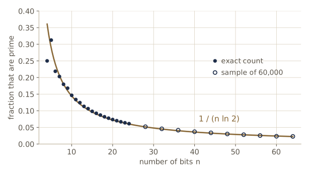
If each candidate is prime with probability \(q\), the number of candidates until the first prime is a geometric random variable with expected value \(1/q\). (If \(E\) is the expected number of tries, then \(E = 1 + (1 - q)E\): we always try once, and with probability \(1 - q\) we start over. So \(E = 1/q\).) With \(q \approx 1.44/n\), we expect about \(0.693n\) candidates. Each costs one primality test, \(O(n^3)\) for a constant number of rounds, so generating an \(n\)-bit prime takes \(O(n^4)\) expected time. Most candidates are cheaper than that, because they fail the first round.
def random_prime(n, rng, test=miller_rabin):
    """A random n-bit prime, and the number of candidates tried."""
    tries = 0
    while True:
        tries += 1
        N = rng.randrange(2 ** (n - 1), 2 ** n)
        if test(N, rng=rng):
            return N, tries

rng = random.Random(11)
print(random_prime(64, rng))
for n in [32, 64, 96, 128]:
    runs = [random_prime(n, rng)[1] for _ in range(400)]
    average = sum(runs) / len(runs)
    print(f"n = {n:3d}   average candidates {average:5.1f}   "
          f"predicted n ln 2 = {n * math.log(2):5.1f}")
(9534946169965397021, 19)
n =  32   average candidates  21.2   predicted n ln 2 =  22.2
n =  64   average candidates  46.3   predicted n ln 2 =  44.4
n =  96   average candidates  66.0   predicted n ln 2 =  66.5
n = 128   average candidates  92.5   predicted n ln 2 =  88.7
The averages track \(n \ln 2\) to within the noise of 400 runs. (Sampling only odd numbers would halve them; exercise 8.)
Which test should random_prime use? Here the input is random, not chosen by an adversary, and random composites are much easier to catch than the worst case suggests. Even a single Fermat round with base 2 is almost always right. The next cell counts, below one million, the composites that pass base 2 — the base-2 pseudoprimes — against the primes.
LIMIT = 10 ** 6
sieve = bytearray([1]) * LIMIT            # sieve of Eratosthenes: the true answer
sieve[0] = sieve[1] = 0
for i in range(2, int(LIMIT ** 0.5) + 1):
    if sieve[i]:
        sieve[i * i::i] = bytearray(len(range(i * i, LIMIT, i)))
passes = [N for N in range(3, LIMIT, 2) if pow(2, N - 1, N) == 1]
pseudo = [N for N in passes if not sieve[N]]
primes = sum(sieve[N] for N in passes)
print(f"odd numbers below 10^6 that pass base 2: {len(passes):,}")
print(f"primes among them: {primes:,}")
print(f"composites that pass: {len(pseudo)}, the first few {pseudo[:5]}")
print(f"chance a passing number is composite: {len(pseudo) / len(passes):.4f}")
odd numbers below 10^6 that pass base 2: 78,742
primes among them: 78,497
composites that pass: 245, the first few [341, 561, 645, 1105, 1387]
chance a passing number is composite: 0.0031
Below a million, only 245 composites slip through against 78,497 odd primes, and the fraction shrinks quickly as the numbers get longer. Numbers that pass a few fixed bases are sometimes called “industrial-grade primes”. For keys, libraries still run several random Miller–Rabin rounds, which cost little next to the search.
Cryptography
The standard setting has three characters. Alice wants to send Bob a message \(x\), which we can take to be a string of bits or a number. She sends an encrypted version \(e(x)\); Bob recovers \(x = d(e(x))\) with a decryption function \(d\). Eve listens to the channel and sees \(e(x)\). The goal is that \(e(x)\) tells Eve nothing useful about \(x\).
For most of history, cryptography was private-key: Alice and Bob agree on a secret in advance and use it to encrypt everything that follows. Eve’s hope is to learn enough about the secret from the messages she intercepts. Public-key cryptography, of which RSA is the classic example, removes the need to meet in advance: Bob publishes a key that lets anyone encrypt messages to him, while only he can decrypt them. That is what lets your browser send a password to a server it has never talked to before.
Private-key schemes: the one-time pad and AES
In the one-time pad, Alice and Bob share a secret random string \(r\) as long as the message. Alice sends \(e_r(x) = x \oplus r\), the bitwise exclusive-or of message and pad. Since \(r \oplus r = 0\), applying the same operation again decrypts: \((x \oplus r) \oplus r = x\). For example, with \(r = 10110100\), the message \(11001010\) encrypts to \(01111110\), and XOR with \(r\) again gives back \(11001010\).
Why is this secure? Suppose Eve intercepts \(y\). For each possible message \(x\), exactly one pad, \(r = x \oplus y\), would have produced \(y\) from \(x\). If \(r\) was chosen uniformly at random from all \(n\)-bit strings, all these pads are equally likely, so from Eve’s point of view every message is equally likely. The ciphertext carries no information at all about \(x\).
def xor(a, b):
    """Bytewise exclusive-or of two equal-length byte strings."""
    return bytes(u ^ v for u, v in zip(a, b))

rng = random.Random(12)
m1, m2 = b"MEET AT THE GYM", b"MEET AT THE LAB"
pad = rng.randbytes(len(m1))
c1, c2 = xor(m1, pad), xor(m2, pad)
print("ciphertext:", c1.hex(), "  decrypted:", xor(c1, pad))
print("c1 XOR c2 :", list(xor(c1, c2)))
ciphertext: 9333382d4a9b8864785615885a2cca   decrypted: b'MEET AT THE GYM'
c1 XOR c2 : [0, 0, 0, 0, 0, 0, 0, 0, 0, 0, 0, 0, 11, 24, 15]
The last line shows why the pad must never be reused. With the same pad for two messages, \(c_1 \oplus c_2 = (m_1 \oplus r) \oplus (m_2 \oplus r) = m_1 \oplus m_2\): the pad cancels, and Eve sees exactly where the messages agree (the zeros) and how they differ. If she can guess one message, she recovers the other. So the pad must be as long as everything Alice and Bob will ever send, which makes it impractical for most uses.
The Advanced Encryption Standard (AES), adopted by the U.S. National Institute of Standards and Technology in 2001, is the widely used alternative. It is also private-key, but the shared secret is short — 128, 192, or 256 bits — and it defines an invertible scrambling of 128-bit blocks that can be reused on block after block. Its security is not proved. It rests on the fact that, despite years of public scrutiny, no one knows how to recover a message from its encryption much faster than by trying all possible keys.
Watch out. Python’s
randommodule is built for simulations, not secrets: from enough of its outputs, the rest can be predicted. Use it (seeded) in these notes so that the outputs are repeatable, but use thesecretsmodule, or a vetted cryptography library, for real keys and pads.
RSA
In RSA each person has a public key, published for the world, and a secret key, known only to them. To send Bob a message, Alice encrypts it with Bob’s public key; Bob decrypts with his secret key. Messages are numbers modulo \(N\) (a long message is cut into pieces). Encryption must be a one-to-one map on \(\{0, 1, \dots, N - 1\}\) so that no information is lost, and decryption is its inverse. RSA’s choice is a power map.
Theorem. Let \(p\) and \(q\) be distinct primes and \(N = pq\). Let \(e\) be relatively prime to \((p-1)(q-1)\), and let \(d\) be the inverse of \(e\) modulo \((p-1)(q-1)\). Then for every \(x \in \{0, 1, \dots, N-1\}\),
\[(x^e)^d \equiv x \pmod N .\]In particular, the map \(x \mapsto x^e \bmod N\) is a bijection on \(\{0, \dots, N - 1\}\), and its inverse is \(y \mapsto y^d \bmod N\).
Proof. The inverse \(d\) exists by the modular division theorem, since \(\gcd(e, (p-1)(q-1)) = 1\). Then \(ed \equiv 1 \pmod{(p-1)(q-1)}\), so \(ed = 1 + k(p-1)(q-1)\) for some integer \(k \ge 0\). We show that \(x^{ed} - x\) is divisible by \(p\). If \(p \mid x\), both terms are multiples of \(p\). Otherwise Fermat’s little theorem gives \(x^{p-1} \equiv 1 \pmod p\), so
\[x^{ed} = x \cdot \left(x^{p-1}\right)^{k(q-1)} \equiv x \cdot 1 = x \pmod p .\]The same argument with the roles of \(p\) and \(q\) swapped shows that \(q\) divides \(x^{ed} - x\). A number divisible by two distinct primes is divisible by their product, so \(N \mid x^{ed} - x\), that is, \((x^e)^d \equiv x \pmod N\). Finally, a map with an inverse is a bijection. \(\square\)
The protocol:
- Key generation (Bob). Pick two random \(n\)-bit primes \(p\) and \(q\) and let \(N = pq\). Pick \(e\) relatively prime to \((p-1)(q-1)\) and compute \(d = e^{-1} \bmod (p-1)(q-1)\) with extended Euclid. Publish \((N, e)\); keep \(d\) (and \(p\), \(q\)) secret.
- Encryption (Alice). Look up \((N, e)\) and send \(y = x^e \bmod N\).
- Decryption (Bob). Compute \(y^d \bmod N\), which is \(x\) by the theorem.
Every step is an algorithm from this module: random prime generation, extended Euclid, and modular exponentiation. A toy example first, with \(p = 13\) and \(q = 19\), so \(N = 247\) and \((p-1)(q-1) = 216\). The exponent \(e = 5\) is relatively prime to 216, and \(d = 5^{-1} \bmod 216 = 173\) (check: \(5 \cdot 173 = 865 = 4 \cdot 216 + 1\)).
def rsa_keys(p, q, e):
    """Public key (N, e) and secret exponent d, for distinct primes p, q."""
    phi = (p - 1) * (q - 1)
    return (p * q, e), inverse(e, phi)

def encrypt(x, public):
    N, e = public
    return pow(x, e, N)

def decrypt(y, public, d):
    N, _ = public
    return pow(y, d, N)

public, d = rsa_keys(13, 19, 5)
y = encrypt(42, public)
print("public key:", public, "  secret d:", d)
print("42 ->", y, "->", decrypt(y, public, d))
images = [encrypt(x, public) for x in range(247)]
print("bijection:", len(set(images)) == 247, "  decrypts every message:",
      all(decrypt(images[x], public, d) == x for x in range(247)))
public key: (247, 5)   secret d: 173
42 -> 74 -> 42
bijection: True   decrypts every message: True
Now at a realistic size: two random 1024-bit primes, a 2048-bit modulus, and the exponent \(e = 65537 = 2^{16} + 1\), a common choice in practice because encrypting with it takes only 17 modular multiplications.
rng = random.Random(2026)
e = 65537
while True:
    p, _ = random_prime(1024, rng)
    q, _ = random_prime(1024, rng)
    if p != q and math.gcd(e, (p - 1) * (q - 1)) == 1:
        break
public, d = rsa_keys(p, q, e)
N = public[0]

message = "Office hours moved to Thursday."
x = int.from_bytes(message.encode(), "big")     # the message as a number below N
y = encrypt(x, public)
back = decrypt(y, public, d)
print(f"N has {N.bit_length()} bits;  x has {x.bit_length()} bits")
print("ciphertext starts:", hex(y)[:34], "...")
print("decrypted:", back.to_bytes((back.bit_length() + 7) // 8, "big").decode())
N has 2048 bits;  x has 247 bits
ciphertext starts: 0x69b11d213e46833f098765191ca6b458 ...
decrypted: Office hours moved to Thursday.
Key generation is the slow part (two prime searches, each expected \(O(n)\) candidates), and it happens once. Encryption and decryption are single modular exponentiations, \(O(n^3)\) each.
Why RSA is believed secure
Eve knows \(N\), \(e\), and \(y = x^e \bmod N\). The security of RSA rests on an assumption:
Assumption. Given \(N\), \(e\), and \(y = x^e \bmod N\) for a random \(x\), no efficient algorithm can find \(x\).
Eve’s obvious strategies fail. She could try every \(x\) until \(x^e \equiv y\), but there are \(N \approx 2^{2n}\) candidates. She could factor \(N\) into \(p\) and \(q\), after which she can compute \(d\) exactly as Bob did — but that requires factoring. For toy keys, factoring is instant; for real keys, trial division is hopeless:
print("247 =", next((k, 247 // k) for k in range(2, 247) if 247 % k == 0))
rng = random.Random(13)
p_small, _ = random_prime(20, rng)
q_small, _ = random_prime(20, rng)
M = p_small * q_small
divisions = is_prime_trial(M)[1]
print(f"{M.bit_length()}-bit N factored after {divisions:,} trial divisions")
247 = (13, 19)
40-bit N factored after 661,420 trial divisions
Each extra bit in the primes doubles that count; for 1024-bit primes it is about \(2^{1024}\). Far better factoring algorithms exist than trial division, but all known ones still take time that grows faster than any polynomial in \(n\), which is why keys of 2048 bits and more are considered safe today. No one has proved that factoring is hard, or that breaking RSA requires factoring. RSA’s insight is to turn a problem nobody can solve into a lock only the key holder can open.
Watch out. The scheme above is “textbook RSA”, and it is not safe to use as is. It is deterministic, so Eve can check a guess of the message by encrypting it herself; and small messages with a small \(e\) can be recovered directly (exercise 10). Real systems first pad the message with random bytes in a carefully specified way. The number theory is the same.
Universal hashing
Our last application of number theory is to a data structure. Suppose a server tracks the currently connected clients, a few hundred of them at any moment, each identified by its IPv4 address, a 32-bit number usually written as four bytes, like 172.16.254.1. We want to insert, delete, and look up addresses quickly. An array indexed by address would give instant lookups but has \(2^{32} \approx 4.3\) billion entries, almost all empty. A plain list of the clients uses little memory but makes each lookup scan the whole list. We want both: memory proportional to the number of clients, and lookups in constant expected time.
Hash tables
A hash table stores items in an array of \(n\) buckets, where \(n\) is about the number of items we expect. A hash function \(h\) maps each possible key to a bucket number in \(\{0, 1, \dots, n-1\}\), and the item with key \(x\) goes in bucket \(h(x)\). Two keys with the same bucket collide; each bucket holds a short list of all the items that hash to it (this is called chaining). To look up \(x\), compute \(h(x)\) and scan that bucket’s list. Memory is \(O(n)\) plus the items, and a lookup costs the time to evaluate \(h\) plus the length of one list. Everything depends on the lists being short.
Why no fixed hash function is safe
A tempting choice is to use one byte of the address, say the last: \(h(x) = x_4\), with 256 buckets. If addresses were uniformly random, this would spread them evenly. Real data are not uniform. Suppose the clients are machines in a few labs, all numbered with small final bytes:
random.seed(14)
# 500 draws of lab addresses 10.20.x.y with a small last byte; duplicates removed
clients = sorted(set((10, 20, random.randrange(256), random.randint(1, 12))
                     for _ in range(500)))
print(len(clients), "clients, e.g.", clients[:3])

def bucket_sizes(keys, h, n):
    sizes = [0] * n
    for x in keys:
        sizes[h(x)] += 1
    return sizes

last_byte = lambda x: x[3]
sizes = bucket_sizes(clients, last_byte, 256)
print("last byte as hash: largest bucket", max(sizes),
      "  nonempty buckets", sum(s > 0 for s in sizes))
458 clients, e.g. [(10, 20, 0, 2), (10, 20, 0, 4), (10, 20, 0, 5)]
last byte as hash: largest bucket 49   nonempty buckets 12
All 458 addresses land in 12 of the 256 buckets, the largest holding 49 of them. Using the first byte would be worse still: every address here starts with 10. The problem is not these particular functions. Every fixed function is bad for some data: with \(2^{32}\) keys and \(n\) buckets, some bucket receives at least \(2^{32}/n\) keys — for \(n = 257\), over 16 million — and if the clients happen to come from that set, they all collide. Whatever \(h\) we fix, some input defeats it.
The way out is the same as in primality testing: randomize. We do not pick one hash function; we pick one at random from a family, when the table is created, and show that for every set of keys, a random member of the family behaves well in expectation. The data cannot be arranged to defeat a function it does not know.
A family built from a prime
Take the number of buckets to be a prime \(n\) larger than every byte value, so \(n > 255\); here \(n = 257\). View a key as a vector \(x = (x_1, x_2, x_3, x_4)\) of numbers modulo \(n\) (each byte is already less than \(n\), and different addresses give different vectors). For every coefficient vector \(a = (a_1, a_2, a_3, a_4)\) with entries in \(\{0, 1, \dots, n-1\}\), define
\[h_a(x_1, x_2, x_3, x_4) = \left(\sum_{i=1}^{4} a_i x_i\right) \bmod n .\]The family is \(\mathcal{H} = \{h_a : a \in \{0, \dots, n-1\}^4\}\), with \(n^4\) members. Choosing a random member means choosing the four coefficients independently and uniformly at random. (The last-byte and first-byte functions are in the family, as \(h_{(0,0,0,1)}\) and \(h_{(1,0,0,0)}\); they are just two of its \(n^4\) members.)
Lemma. For any two distinct keys \(x \ne y\), if \(a\) is chosen uniformly at random, then \(\Pr[h_a(x) = h_a(y)] = 1/n\).
Proof. Since \(x \ne y\), they differ in some coordinate; renumbering if needed, say \(x_4 \ne y_4\). The two keys collide exactly when \(\sum_i a_i x_i \equiv \sum_i a_i y_i \pmod n\), which rearranges to
\[a_4 (x_4 - y_4) \equiv \sum_{i=1}^{3} a_i (y_i - x_i) \pmod n .\]Imagine drawing \(a_1, a_2, a_3\) first. The right-hand side is then some fixed number \(c\). Because \(n\) is prime and \(x_4 - y_4 \not\equiv 0 \pmod n\), the difference \(x_4 - y_4\) has an inverse modulo \(n\), so the congruence holds for exactly one value of \(a_4\), namely \(c \cdot (x_4 - y_4)^{-1} \bmod n\). The last coefficient is uniform over \(n\) values, so it hits that one value with probability \(1/n\), whatever \(a_1, a_2, a_3\) were. \(\square\)
A collision probability of \(1/n\) is what we would get if each key were sent to an independent, uniformly random bucket — the ideal — but here it comes from a function that is consistent (the same key always goes to the same bucket) and cheap to evaluate. This is the property we name:
Definition. A family \(\mathcal{H}\) of hash functions into \(n\) buckets is universal if, for any two distinct keys \(x \ne y\), exactly \(\lvert \mathcal{H} \rvert / n\) of the functions in \(\mathcal{H}\) map \(x\) and \(y\) to the same bucket. Equivalently, a random \(h \in \mathcal{H}\) makes them collide with probability \(1/n\).
For small parameters we can check the definition exhaustively: with \(n = 5\) and keys of length 3, there are \(125\) keys, \(7{,}750\) pairs of keys, and \(125\) functions, and each pair should collide under exactly \(125/5 = 25\) of them.
from itertools import product, combinations

def h(a, x, n):
    """The hash function h_a applied to key x: sum of a_i * x_i, mod n."""
    return sum(ai * xi for ai, xi in zip(a, x)) % n

n, k = 5, 3
keys = list(product(range(n), repeat=k))
family = list(product(range(n), repeat=k))
counts = set()
for x, y in combinations(keys, 2):
    counts.add(sum(h(a, x, n) == h(a, y, n) for a in family))
print(f"{len(keys)} keys, {len(family)} functions;",
      f"collisions per pair take the values {counts}")
125 keys, 125 functions; collisions per pair take the values {25}
Every pair collides under exactly 25 functions, as the lemma says. At the real size we sample instead: one fixed pair of addresses and many random functions with \(n = 257\).
rng = random.Random(15)
n = 257
x, y = (10, 20, 7, 3), (10, 20, 8, 3)                 # two neighboring lab machines
trials = 200_000
hits = 0
for _ in range(trials):
    a = [rng.randrange(n) for _ in range(4)]
    hits += h(a, x, n) == h(a, y, n)
print(f"collision frequency {hits / trials:.5f}   1/n = {1 / n:.5f}")
collision frequency 0.00399 1/n = 0.00389
What universality buys: short buckets
Put \(m\) keys in a table of \(n\) buckets using a random \(h\) from a universal family, and consider looking up a key \(x\) (in the table or not). The cost is the length of \(x\)’s bucket. For each other key \(y_j\) in the table, let \(Y_j\) be 1 if \(y_j\) collides with \(x\) and 0 otherwise; then \(\mathbb{E}[Y_j] = \Pr[Y_j = 1] = 1/n\). The number of other keys in \(x\)’s bucket is \(Y = \sum_j Y_j\), and by linearity of expectation — the expected value of a sum is the sum of the expected values, whether or not the terms are independent —
\[\mathbb{E}[Y] = \sum_{j} \mathbb{E}[Y_j] \le \frac{m}{n} .\]So the expected bucket length is at most \(1 + m/n\). With \(n\) at least the number of keys, that is at most 2, and a lookup, insertion, or deletion takes constant expected time — for every set of keys, the adversarial ones included. The ratio \(m/n\) is called the load factor.
rng = random.Random(16)
n = 257
for trial in range(3):
    a = [rng.randrange(n) for _ in range(4)]
    sizes = bucket_sizes(clients, lambda x: h(a, x, n), n)
    seen = sum(s * s for s in sizes) / len(clients)   # mean size of a key's bucket
    print(f"a = {a}:  largest bucket {max(sizes)},",
          f"average bucket seen by a key {seen:.2f}")
print(f"bound 1 + (m-1)/n = {1 + (len(clients) - 1) / n:.2f}")
a = [185, 240, 246, 145]:  largest bucket 6, average bucket seen by a key 2.65
a = [213, 116, 228, 2]:  largest bucket 5, average bucket seen by a key 2.54
a = [209, 132, 121, 113]:  largest bucket 6, average bucket seen by a key 2.53
bound 1 + (m-1)/n = 2.78
The same lab addresses that piled 49 deep under the last-byte hash now spread out: the largest bucket holds 5 or 6 keys, and a key’s bucket has about 2.5 to 2.7 keys on average, within the bound \(1 + (m-1)/n \approx 2.78\) (the load factor here is \(458/257 \approx 1.8\)). A table of about twice as many buckets would bring the average down toward 1.5.
Using it in general
The recipe works for any kind of key:
- Choose the table size \(n\) to be a prime a little larger than the number of items you expect — about twice as large keeps buckets short. There is always a prime between \(m\) and \(2m\), and random search with a primality test finds one quickly.
- Cut each key into \(k\) pieces, each a number less than \(n\) (for example, \(\lfloor \log n \rfloor\) bits at a time), so a key becomes a vector in \(\{0, \dots, n-1\}^k\).
- When the table is created, choose \(a_1, \dots, a_k\) at random, and hash with \(h_a(x) = \sum a_i x_i \bmod n\).
The universality proof carries over word for word: two distinct keys differ in some piece, and the coefficient of that piece is uniform. Evaluating \(h_a\) costs \(k\) multiplications of \(O(\log n)\)-bit numbers.
Note. Python’s built-in
hashfor strings and bytes is salted with a random value chosen when the interpreter starts, so the same string gets different hash values in different runs (comparepython3 -c "print(hash('abc'))"twice). The motivation is the one above: an attacker who knows the hash function can send keys that all collide and slow a server’s dictionaries to a crawl.
Summary
| Problem | Algorithm | Running time (\(n\)-bit inputs) |
|---|---|---|
| Addition | grade-school, column by column with a carry | \(O(n)\), optimal |
| Multiplication | grade-school, or the halving rule | \(O(n^2)\) (faster in module 02) |
| Division with remainder | halving rule, one correction per bit | \(O(n^2)\) |
| Modular addition / multiplication | ordinary operation, then reduce | \(O(n)\) / \(O(n^2)\) |
| Modular exponentiation \(x^y \bmod N\) | repeated squaring | \(O(n^3)\) |
| \(\gcd(a, b)\) | Euclid’s algorithm | \(O(n)\) calls, \(O(n^3)\) |
| Coefficients with \(ax + by = \gcd(a, b)\); inverse mod \(N\) | extended Euclid | \(O(n^3)\) |
| Primality | Fermat or Miller–Rabin test, \(k\) random bases | \(O(kn^3)\), error at most \(2^{-k}\) (Fermat, non-Carmichael) or \(4^{-k}\) (Miller–Rabin) |
| Random \(n\)-bit prime | sample and test | expected \(O(n)\) candidates, \(O(n^4)\) time |
| RSA key generation / encryption / decryption | random primes, extended Euclid, modular exponentiation | expected \(O(n^4)\) / \(O(n^3)\) / \(O(n^3)\) |
| Hash-table operation | random member of a universal family, chaining | expected \(O(1 + m/n)\) bucket length |
Ideas to carry forward:
- Measure input size in bits. An algorithm that loops once per unit of a number’s value (trial division, naive exponentiation) is exponential; one that loops once per bit (halving, squaring, Euclid) is polynomial.
- Reducing modulo \(N\) at every step keeps numbers small without changing the answer, and inverses exist exactly for numbers relatively prime to \(N\).
- Randomization can make an algorithm reliable against every input: a one-sided error of at most \(1/2\) per round becomes \(2^{-k}\) after \(k\) rounds, and a randomly chosen hash function cannot be defeated by the data.
- The gap between an easy problem (primality) and a hard one (factoring) can be put to work, as RSA does.
Exercises
- Show that \(H_N = 1 + \tfrac12 + \dots + \tfrac1N\) satisfies \(\tfrac12 \lfloor \log N \rfloor \le H_N \le \lfloor \log N \rfloor + 1\) by grouping the terms into blocks \([2^j, 2^{j+1})\). Conclude that \(H_N = \Theta(\log N)\).
- Write
subtract(x, y)for bit lists with \(x \ge y\) (the borrow method) andcompare(x, y), each in \(O(n)\) bit operations. Use them to implementdivideentirely on bit lists, count its bit operations for random \(n\)-bit inputs with \(n = 64, 128, 256, 512\), and check that the counts grow like \(n^2\). - Suppose \(x\) has \(n\) bits and \(y\) has \(m\) bits. How many bit operations does
multiply(x, y)use, as a function of both \(n\) and \(m\)? Does it matter which argument is halved? Verify your answer by counting. - Without a computer, find \((5^{1000} + 6^{1000}) \bmod 7\) and the last decimal digit of \(7^{2026}\). Show the reductions you use. Then check your answers with
pow. - Prove that if \(a\) has a multiplicative inverse modulo \(N\), the inverse is unique modulo \(N\). Then show that exactly \(2^{k-1}\) of the numbers \(0, 1, \dots, 2^k - 1\) are invertible modulo \(2^k\).
- Run extended Euclid by hand on \((89, 55)\), two consecutive Fibonacci numbers, and find \(55^{-1} \bmod 89\). What pattern do the coefficients follow? State and prove a general formula for
extended_euclid(F(k+1), F(k)). - Show that \(2465 = 5 \cdot 17 \cdot 29\) is a Carmichael number without trying all bases, by the argument used in the notes for \((6k+1)(12k+1)(18k+1)\). Then write a program that finds all Carmichael numbers below 100,000 (make it fast enough by testing only bases up to a few hundred, plus a correct final check), and observe that each has at least three prime factors.
- (a) Prove that if \(x^2 \equiv 1 \pmod N\) but \(x \not\equiv \pm 1 \pmod N\), then \(\gcd(x - 1, N)\) is a factor of \(N\) strictly between 1 and \(N\). (b) Modify
miller_rabinso that, when it finds a nontrivial square root of 1, it returns a factor of \(N\); test it on 561, 1105, and 1729. (c) Modifyrandom_primeto sample only odd candidates, predict the new expected number of candidates, and measure it. - Bob’s RSA key has \(p = 23\), \(q = 29\), and \(e = 3\). Find \(d\) by hand with extended Euclid. Encrypt the message \(x = 100\), and decrypt the result using \(d\). Why would \(e = 7\) not be a valid choice here?
- Suppose Bob uses \(e = 3\) and Alice encrypts a message \(x\) with \(x^3 < N\). Show that Eve can recover \(x\) from \(y\) without factoring \(N\), and implement the attack with an integer cube root computed by binary search. Test it on the 2048-bit key from the notes with \(e = 3\) (generate new primes so that \(\gcd(3, (p-1)(q-1)) = 1\)).
- The family in the notes needs every piece of a key to be less than the prime \(n\). Suppose instead that keys are 4-byte addresses but \(n = 251\). Find two distinct addresses that collide under every \(h_a\), and explain which step of the universality proof fails. What is the smallest prime that works for byte-sized pieces?
- In your own words: explain to a classmate why primality testing is easy while factoring is believed hard, even though knowing the factors of \(N\) would immediately tell you whether \(N\) is prime. Your answer should say what the Fermat or Miller–Rabin test learns about \(N\) when it declares it composite, and what it does not learn.
Going further
- Dasgupta, Papadimitriou, and Vazirani, Algorithms, chapter 1 — the source for this module. Exercises 1.9–1.13 practice modular arithmetic, 1.20–1.28 inverses and RSA, 1.29 asks which hash families are universal, 1.36–1.37 cover square roots modulo a prime and the Chinese remainder theorem, and 1.45–1.46 build digital signatures from RSA.
- R. L. Rivest, A. Shamir, and L. Adleman, “A method for obtaining digital signatures and public-key cryptosystems”, Communications of the ACM, 1978 — the original RSA paper, short and readable.
- J. L. Carter and M. N. Wegman, “Universal classes of hash functions”, Journal of Computer and System Sciences, 1979 — where universal hashing was introduced.
- M. Agrawal, N. Kayal, and N. Saxena, “PRIMES is in P”, Annals of Mathematics, 2004 — the deterministic polynomial-time primality test.
- Python documentation: the built-in
pow(includingpow(a, -1, N)for inverses) and thesecretsmodule for cryptographic randomness.
These notes follow the chapters of S. Dasgupta, C. H. Papadimitriou, and U. V. Vazirani, Algorithms (McGraw-Hill, 2008), the course text. The explanations, code, figures, and exercises here are written for this course; the book remains the reference, with many more exercises.