EAS 510 · Module 08 · Week 9
Replicating a Research Paper
Reading a paper as a set of equations and a figure, and turning it into code — the Vision Transformer, piece by piece.
Companion reading: Learn PyTorch for Deep Learning, chapter 08
By the end of this module you can
- Explain what paper replicating is, name the usual sections of a machine learning paper, and read one in three passes.
- Translate a paper’s architecture figure, equations, and hyperparameter table into PyTorch layers, checking the shape after every step.
- Build the Vision Transformer’s patch embedding, class token, and position embeddings (equation 1).
- Explain in plain words what self-attention does, and build the attention and MLP blocks with LayerNorm and residual connections (equations 2 and 3).
- Assemble a complete ViT-Base, verify its parameter count, and compare your encoder block with
torch.nn.TransformerEncoderLayer. - Diagnose why a Vision Transformer trained from scratch on a few hundred images performs poorly, and list what the paper’s training recipe adds.
- Use a pretrained ViT-B/16 from torchvision as a feature extractor, save it, and weigh its file size for deployment.
Contents
- What paper replicating is
- Reading a machine learning paper
- Setting up
- The Vision Transformer at a glance
- Equation 1: turning an image into a sequence
- Equation 2: the attention block
- Equation 3: the MLP block
- The Transformer encoder block
- Putting it together: the full ViT
- Training our ViT from scratch
- A pretrained ViT as a feature extractor
- Summary
- Exercises
- Going further
So far every architecture we used was either small enough to write from memory (TinyVGG in module 04) or came ready-made from torchvision (module 06). In module 07 we compared several of those ready-made models with evidence. This module takes the next step: we start from a research paper — a PDF of text, one diagram, a handful of equations, and some tables — and turn it into working PyTorch code.
The paper is Dosovitskiy et al., 2020, An Image is Worth 16x16 Words: Transformers for Image Recognition at Scale, which introduced the Vision Transformer (ViT). We will build it one equation at a time, check every tensor shape against the paper as we go, train it on our pizza, steak, and sushi images, find out why that goes badly, and fix it with a pretrained version.
The ViT itself matters — Transformer models now sit behind much of modern computer vision and most of modern language processing — but the lasting skill is the method: reading a paper, breaking it into inputs, outputs, layers, and blocks, and writing each piece as code you can test.
What paper replicating is
New methods in machine learning appear first as research papers. Paper replicating means turning a paper’s figures, math, and text into code that behaves the way the paper describes, so you can use the method on your own problem.
Why is it a core skill?
- The method you need may exist only on paper. Code is not always released, and when it is, it may not fit your data, your framework, or your hardware.
- It forces real understanding. You cannot write a layer you have not understood; every vague sentence in the paper becomes a concrete question about a shape or a number.
- It is how the field stays usable. Libraries such as
torchvision, Hugging Face Transformers, andtimmexist largely because people replicated papers and shared the code.
If you have ever implemented a method from a journal article in your own simulation or analysis code — a new filter for sensor data, a material model, a fatigue criterion — you have already done this. The machine learning version has the same shape: find the parts of the paper that define the method, translate each into code, and check each piece before you trust the whole.
Reading a machine learning paper
The anatomy of a paper
Most machine learning papers follow a similar layout. Each section answers a different question, and when you replicate, you use them differently.
| Section | What it tells you | What you take from it when replicating |
|---|---|---|
| Abstract | The main claim in one paragraph | Whether the paper is worth your time |
| Introduction | The problem, earlier approaches, and what is new | Why the method looks the way it does |
| Method | The model, the data, and how it is trained | The figure and equations you will turn into code |
| Results (experiments) | How the method compares with earlier ones | The numbers you would try to reproduce, and the hyperparameter tables |
| Conclusion | Limitations and next steps | Where the method may not suit your problem |
| References | The earlier work it builds on | Papers to read when a detail is left unexplained |
| Appendix | Details that did not fit in the main text | Often the training details you need — for ViT, where dropout goes and which optimizer settings to use |
| Code | A link to the authors’ implementation, when released | A reference to check your own version against |
Reading in three passes
A useful habit, from S. Keshav’s short note How to Read a Paper, is to read a paper in three passes rather than once from top to bottom.
- First pass (5–10 minutes). Read the title, abstract, and introduction, glance at the section headings and figures, and read the conclusion. Decide whether the paper is relevant and what kind of contribution it makes.
- Second pass (about an hour). Read the whole paper carefully but skip long derivations. Study the figures and tables. Note terms you don’t know and references you may need. For a replication, this is when you mark the architecture figure, the equations, and the hyperparameter tables.
- Third pass (several hours). Rebuild the work yourself. For us this means writing code, one piece at a time, and checking each piece against the paper.
For the ViT paper, the second pass points to three places that define the model: Figure 1 (the architecture diagram), the four equations in Section 3.1, and Table 1 (the sizes of the model variants). Training details are in Table 3 and Appendix B.1.
Layers, blocks, and a replicating workflow
A whole paper is intimidating; a single layer is not. So we break the model into pieces:
- A layer takes an input tensor, applies one operation (a convolution, a normalization, a linear map), and returns an output tensor.
- A block is a small group of layers that together do one job, and it also takes an input and returns an output.
- The architecture (the model) is a stack of blocks.
The workflow for the rest of this module:
- For each piece, write down its input and output shapes before writing code.
- Build the piece with existing PyTorch layers where possible.
- Pass a real tensor through it and check the output shape against step 1.
- Combine pieces into blocks, and blocks into the model. Build the smallest version described in the paper first (for ViT, ViT-Base).
- When stuck, compare with other implementations:
torchvision’s ownvision_transformer.py, orvit-pytorch, a collection of Vision Transformer variants written in PyTorch.
Papers themselves are easy to find: arXiv hosts free preprints of most machine learning papers, Hugging Face Papers lists new ones daily with links to code and models, and the major conferences (NeurIPS, ICML, ICLR — where the ViT paper was published) put their proceedings online.
Setting up
We reuse the going_modular package from module 05. We will also use torchinfo to print model summaries; Colab does not include it, so install it first:
!pip install -q torchinfo
import matplotlib.pyplot as plt
import torch
import torchvision
from torch import nn
from torchvision import transforms
from torchinfo import summary

print(f"torch version: {torch.__version__}")
print(f"torchvision version: {torchvision.__version__}")
torch version: 2.14.0+cu130
torchvision version: 0.29.0+cu130
If you still have your going_modular folder from module 05, upload it to Colab. Otherwise this cell downloads the reference copies of the scripts:
import requests
from pathlib import Path

Path("going_modular").mkdir(exist_ok=True)
base = "https://raw.githubusercontent.com/mrdbourke/pytorch-deep-learning/main/going_modular/going_modular/"
for name in ["data_setup.py", "engine.py", "model_builder.py", "utils.py"]:
    path = Path("going_modular") / name
    if not path.exists():
        path.write_text(requests.get(base + name).text)

from going_modular import data_setup, engine, utils
device = "cuda" if torch.cuda.is_available() else "cpu"
device
'cpu'
The pizza, steak, and sushi images
We continue with the three-class food dataset from modules 04–07: about 75 training images and 25 test images per class.
import io
import zipfile

data_path = Path("data")
image_path = data_path / "pizza_steak_sushi"

if image_path.is_dir():
    print(f"{image_path} already exists, skipping download.")
else:
    url = "https://raw.githubusercontent.com/mrdbourke/pytorch-deep-learning/main/data/pizza_steak_sushi.zip"
    image_path.mkdir(parents=True, exist_ok=True)
    with zipfile.ZipFile(io.BytesIO(requests.get(url).content)) as zip_file:
        zip_file.extractall(image_path)
    print(f"Downloaded and unzipped images to {image_path}")

train_dir = image_path / "train"
test_dir = image_path / "test"
data/pizza_steak_sushi already exists, skipping download.
The first reference to the paper comes already. Table 3 lists the training resolution as 224, so we resize every image to 224 × 224 pixels. The paper trained with a batch size of 4,096 images; that needs far more memory than a free Colab GPU has, so we keep our usual 32. Since we train from scratch first, we don’t normalize the images the way a pretrained model would expect.
IMG_SIZE = 224      # "Training resolution is 224" (Table 3)
BATCH_SIZE = 32     # the paper used 4096

manual_transforms = transforms.Compose([
    transforms.Resize((IMG_SIZE, IMG_SIZE)),
    transforms.ToTensor(),
])

train_dataloader, test_dataloader, class_names = data_setup.create_dataloaders(
    train_dir=train_dir,
    test_dir=test_dir,
    transform=manual_transforms,
    batch_size=BATCH_SIZE,
)
print(f"Classes: {class_names}")
print(f"Batches of {BATCH_SIZE}: {len(train_dataloader)} train, {len(test_dataloader)} test")
Classes: ['pizza', 'steak', 'sushi']
Batches of 32: 8 train, 3 test
We will follow one image through every piece of the model:
image, label = train_dataloader.dataset[1]      # one pizza photo from the training set
print(f"Image shape: {image.shape} -> [color_channels, height, width]")
print(f"Label: {label} ({class_names[label]})")
Image shape: torch.Size([3, 224, 224]) -> [color_channels, height, width]
Label: 0 (pizza)
The Vision Transformer at a glance
The Transformer was introduced in 2017 in Attention Is All You Need (Vaswani et al.) for translating text. A Transformer is a network whose main building block is attention, a layer that lets every element of a sequence gather information from every other element — in the way that a convolutional network’s main building block is the convolution. A text Transformer reads a sentence as a sequence of tokens (roughly, words), each represented by a vector of numbers.
The ViT’s idea fits in its title: cut an image into 16 × 16-pixel patches and treat each patch as a word. Once an image is a sequence of patch vectors, the standard Transformer can process it almost unchanged.
Figure 1: the architecture
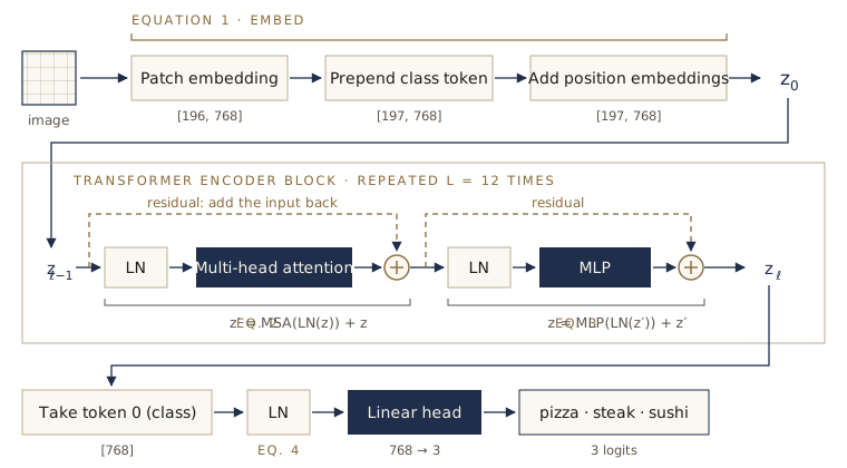
Open the paper and look at Figure 1 alongside this section. Its left half shows an image cut into patches, each patch flattened and passed through a “linear projection”, an extra learnable “class” token placed in front, position embeddings added, the sequence passed through a “Transformer Encoder”, and an “MLP Head” producing the class. Its right half zooms into one encoder block: Norm, Multi-Head Attention, a “+”, Norm, MLP, another “+”, repeated L times.
Our own diagram of the same architecture, labeled with the equation that describes each part:
The four equations
Section 3.1 of the paper describes the model in four equations. Here they are, followed by what each symbol means. The letter \(\mathbf{z}\) is the sequence of token vectors at some point in the network.
Equation 1 — build the input sequence:
\[\mathbf{z}_0 = \left[\mathbf{x}_\text{class};\, \mathbf{x}_p^1\mathbf{E};\, \mathbf{x}_p^2\mathbf{E};\, \cdots;\, \mathbf{x}_p^N\mathbf{E}\right] + \mathbf{E}_{pos}, \qquad \mathbf{E} \in \mathbb{R}^{(P^2 \cdot C) \times D},\ \ \mathbf{E}_{pos} \in \mathbb{R}^{(N+1) \times D}\]Here \(\mathbf{x}_p^i\) is the \(i\)-th patch flattened into a list of \(P^2 \cdot C\) numbers (\(P\) is the patch size, \(C\) the number of color channels), \(\mathbf{E}\) is a learned matrix that maps each patch to a vector of length \(D\), \(\mathbf{x}_\text{class}\) is a learned class token, the square brackets with semicolons mean “stack these into one sequence”, and \(\mathbf{E}_{pos}\) holds one learned position vector per slot in the sequence.
Equation 2 — the attention half of an encoder block:
\[\mathbf{z}'_\ell = \operatorname{MSA}\left(\operatorname{LN}\left(\mathbf{z}_{\ell-1}\right)\right) + \mathbf{z}_{\ell-1}, \qquad \ell = 1, \ldots, L\]LN is layer normalization, MSA is multi-head self-attention, \(\ell\) counts the blocks from 1 to \(L\), and adding \(\mathbf{z}_{\ell-1}\) at the end is a residual connection. All three are explained when we build them.
Equation 3 — the MLP half of an encoder block:
\[\mathbf{z}_\ell = \operatorname{MLP}\left(\operatorname{LN}\left(\mathbf{z}'_\ell\right)\right) + \mathbf{z}'_\ell, \qquad \ell = 1, \ldots, L\]Equation 4 — the output:
\[\mathbf{y} = \operatorname{LN}\left(\mathbf{z}_L^0\right)\]\(\mathbf{z}_L^0\) is token number 0 — the class token — after the last block. The paper then passes \(\mathbf{y}\) to a classification head: a small MLP during pretraining, a single linear layer during fine-tuning. We use a single linear layer.
Read as code, the four equations are short:
| Equation | In words | As code (a sketch) |
|---|---|---|
| 1 | cut into patches and project, prepend the class token, add positions | x = torch.cat([cls, patch_embed(img)], dim=1) + pos |
| 2 | normalize, attend, add the input back | x = msa(ln(x)) + x |
| 3 | normalize, MLP, add the input back | x = mlp(ln(x)) + x |
| 4 | normalize the class token’s output, then classify | y = head(ln(x[:, 0])) |
Table 1: how big
Table 1 gives the sizes of three variants:
| Model | Layers (L) | Hidden size (D) | MLP size | Heads | Parameters |
|---|---|---|---|---|---|
| ViT-Base | 12 | 768 | 3072 | 12 | 86M |
| ViT-Large | 24 | 1024 | 4096 | 16 | 307M |
| ViT-Huge | 32 | 1280 | 5120 | 16 | 632M |
- Layers — how many encoder blocks are stacked.
- Hidden size D — the length of every token vector throughout the model, also called the embedding dimension.
- MLP size — the number of hidden units inside each MLP block.
- Heads — how many attention heads each attention layer has.
We replicate ViT-Base with 16 × 16 patches, which the paper calls ViT-B/16. Start with the smallest version; the same code scales to the others by changing four numbers.
Equation 1: turning an image into a sequence
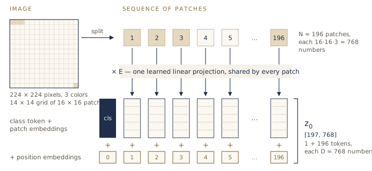
Section 3.1 opens with the recipe: reshape an image of size \(H \times W \times C\) into a sequence of \(N = HW/P^2\) flattened patches, each of length \(P^2 \cdot C\), and map each one to \(D\) numbers with a trainable linear projection. The results are the patch embeddings. An embedding is a learned vector representation of something — here, of a patch. “Learned” is the important word: the numbers start random and improve during training.
Shapes by hand
Before writing any layers, work out the shapes with ViT-B/16’s numbers:
height, width = 224, 224    # H, W
color_channels = 3          # C
patch_size = 16             # P

number_of_patches = (height * width) // patch_size**2
print(f"Number of patches N = HW / P^2 = {number_of_patches}")
print(f"Input shape (one image):       {(height, width, color_channels)}")
print(f"Output shape (patch sequence): {(number_of_patches, patch_size**2 * color_channels)}")
Number of patches N = HW / P^2 = 196
Input shape (one image):       (224, 224, 3)
Output shape (patch sequence): (196, 768)
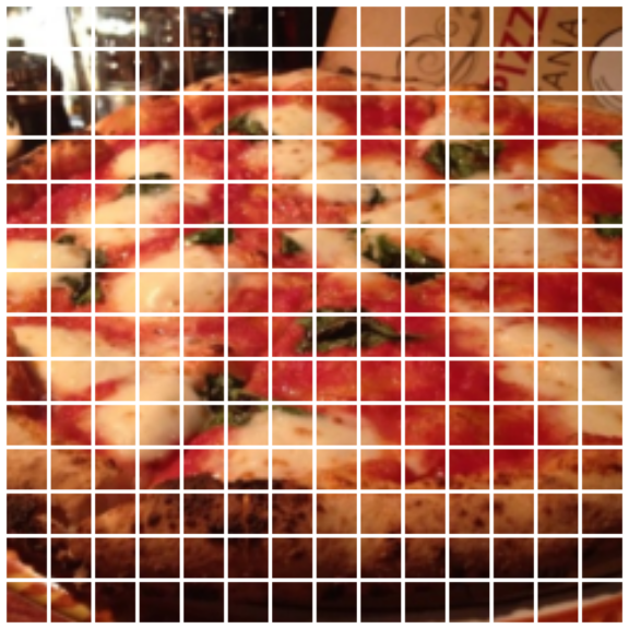
A 224 × 224 image is a 14 × 14 grid of 16 × 16 patches: 196 patches, each holding \(16 \times 16 \times 3 = 768\) numbers. That is our target: a (196, 768) sequence.
Note. For ViT-B/16 two different numbers happen to be equal: a flattened patch has \(P^2 \cdot C = 768\) values, and the embedding size \(D\) is also 768. They are not the same thing. With 32 × 32 patches, a flattened patch has 3,072 values, but ViT-Base still projects it to \(D = 768\).
Seeing the patches
Before building the layer, look at what “cutting into patches” means for our pizza. Each patch is a slice of the image tensor: rows i*16 to (i+1)*16 and columns j*16 to (j+1)*16.
image_permuted = image.permute(1, 2, 0)          # [H, W, C], the order matplotlib expects
patches_per_side = IMG_SIZE // patch_size        # 14

fig, axs = plt.subplots(nrows=patches_per_side, ncols=patches_per_side, figsize=(6, 6))
for i in range(patches_per_side):                # patch rows
    for j in range(patches_per_side):            # patch columns
        patch = image_permuted[i * patch_size:(i + 1) * patch_size,
                               j * patch_size:(j + 1) * patch_size, :]
        axs[i, j].imshow(patch)
        axs[i, j].axis("off")
plt.show()
The patch embedding is a convolution
Looping over patches is fine for a picture but slow for a model. There is a neater way. Recall the convolution from module 03: a small kernel slides over the image and computes a weighted sum at each position. If the kernel is exactly one patch in size (16 × 16) and it moves exactly one patch at a time (stride 16), each position of the kernel covers one whole patch, with no overlap. A weighted sum of a patch’s 768 numbers, plus a bias, is exactly one output of a linear projection. With 768 kernels, each patch gets 768 outputs: its patch embedding.
The paper hints at this too. Its “hybrid architecture” paragraph describes building the input sequence by flattening a CNN’s feature map and projecting it.
torch.manual_seed(42)
conv2d = nn.Conv2d(in_channels=3,           # color channels
                   out_channels=768,        # D from Table 1: one kernel per embedding number
                   kernel_size=patch_size,  # each kernel covers one whole patch...
                   stride=patch_size,       # ...and jumps one whole patch at a time
                   padding=0)

image_out_of_conv = conv2d(image.unsqueeze(0))   # unsqueeze adds a batch dimension
print(f"Output shape: {image_out_of_conv.shape} -> [batch, embedding_dim, patch_rows, patch_cols]")
Output shape: torch.Size([1, 768, 14, 14]) -> [batch, embedding_dim, patch_rows, patch_cols]
Each of the 14 × 14 positions now holds 768 numbers — one embedding per patch. Don’t take the claim on trust; check it against the equation. Flatten the top-left patch by hand, multiply it by the convolution’s weights arranged as a matrix, and compare with what the convolution produced at position (0, 0):
first_patch = image[:, :patch_size, :patch_size]      # top-left patch, [3, 16, 16]
flat_patch = first_patch.flatten()                     # x_p^1: 768 numbers
E = conv2d.weight.reshape(768, -1)                     # the projection as a matrix: [768, 768]
by_hand = E @ flat_patch + conv2d.bias                 # multiply by the matrix, add the bias
from_conv = image_out_of_conv[0, :, 0, 0]              # the convolution's output for that patch

print(f"Flattened patch: {flat_patch.shape}, E: {E.shape}")
print(f"Same result: {torch.allclose(by_hand, from_conv, atol=1e-5)}")
Flattened patch: torch.Size([768]), E: torch.Size([768, 768])
Same result: True
The convolution is the matrix \(\mathbf{E}\) of equation 1, applied to every patch at once. (PyTorch stores it with rows and columns swapped compared with the paper, the same convention nn.Linear uses; the arithmetic is identical.)
Flattening into a sequence
We have [1, 768, 14, 14] and want [1, 196, 768]. First merge the two grid dimensions into one with nn.Flatten, telling it to flatten only dimensions 2 and 3:
flatten = nn.Flatten(start_dim=2, end_dim=3)    # flatten only the 14 x 14 grid
image_out_of_conv_flattened = flatten(image_out_of_conv)
print(f"After flatten: {image_out_of_conv_flattened.shape} -> [batch, embedding_dim, num_patches]")

patch_sequence = image_out_of_conv_flattened.permute(0, 2, 1)
print(f"After permute: {patch_sequence.shape} -> [batch, num_patches, embedding_dim]")
After flatten: torch.Size([1, 768, 196]) -> [batch, embedding_dim, num_patches]
After permute: torch.Size([1, 196, 768]) -> [batch, num_patches, embedding_dim]
The permute puts the sequence dimension before the embedding dimension, which is the order the Transformer layers expect: one row per token.
A PatchEmbedding layer
Wrap the two steps in an nn.Module so the rest of the model can use them as a single layer. The check at the top of forward catches images whose size is not a multiple of the patch size.
class PatchEmbedding(nn.Module):
    """Turns a 2D image into a sequence of learnable patch embeddings.

    Args:
        in_channels: number of color channels in the image.
        patch_size: height and width of each square patch.
        embedding_dim: length D of each patch embedding.
    """
    def __init__(self, in_channels: int = 3, patch_size: int = 16, embedding_dim: int = 768):
        super().__init__()
        self.patch_size = patch_size
        self.patcher = nn.Conv2d(in_channels=in_channels,
                                 out_channels=embedding_dim,
                                 kernel_size=patch_size,
                                 stride=patch_size,
                                 padding=0)
        self.flatten = nn.Flatten(start_dim=2, end_dim=3)

    def forward(self, x):
        image_resolution = x.shape[-1]
        assert image_resolution % self.patch_size == 0, \
            f"Input image size must be divisible by patch size, image shape: {image_resolution}, patch size: {self.patch_size}"
        x_patched = self.patcher(x)                 # [batch, D, rows, cols]
        x_flattened = self.flatten(x_patched)       # [batch, D, N]
        return x_flattened.permute(0, 2, 1)         # [batch, N, D]
torch.manual_seed(42)
patchify = PatchEmbedding(in_channels=3, patch_size=16, embedding_dim=768)

patch_embedded_image = patchify(image.unsqueeze(0))
print(f"Input shape:  {image.unsqueeze(0).shape}")
print(f"Output shape: {patch_embedded_image.shape}")
Input shape:  torch.Size([1, 3, 224, 224])
Output shape: torch.Size([1, 196, 768])
And the check does its job on an image that cannot be cut evenly:
patchify(torch.randn(1, 3, 250, 250))
AssertionError: Input image size must be divisible by patch size, image shape: 250, patch size: 16
The class token
The paper borrows an idea from BERT, a Transformer for text: “we prepend a learnable embedding to the sequence of embedded patches”, and its state at the end of the encoder “serves as the image representation”. The class token is one extra vector, the same for every image, placed at position 0. It holds no pixels. As the sequence passes through the attention layers it gathers information from all the patches, and at the end the classifier reads only this token.
It must be learnable, so we wrap it in nn.Parameter — the same wrapper that makes a layer’s weights trainable — and join it to the front of the sequence with torch.cat along dimension 1, the sequence dimension:
batch_size = patch_embedded_image.shape[0]
embedding_dimension = patch_embedded_image.shape[-1]

class_token = nn.Parameter(torch.randn(batch_size, 1, embedding_dimension),
                           requires_grad=True)
print(f"Class token shape: {class_token.shape} -> [batch, 1 token, embedding_dim]")

patch_embedded_image_with_class_token = torch.cat((class_token, patch_embedded_image), dim=1)
print(f"Sequence with class token: {patch_embedded_image_with_class_token.shape}")
Class token shape: torch.Size([1, 1, 768]) -> [batch, 1 token, embedding_dim]
Sequence with class token: torch.Size([1, 197, 768])
196 patch tokens plus one class token: 197 tokens.
Position embeddings
Attention, as we will see, compares every token with every other token, and the comparison does not depend on where tokens sit in the sequence. Shuffle the patches and the attention layer computes the same thing for each of them. But position matters in an image: sky is usually above ground. Position embeddings fix this by adding a different learned vector to each slot, so the same patch content looks slightly different at position 5 than at position 150.
The paper uses “standard learnable 1D position embeddings” — one vector per slot, shape \((N + 1) \times D\) — and reports that fancier 2D-aware versions did not help.
position_embedding = nn.Parameter(torch.randn(1, number_of_patches + 1, embedding_dimension),
                                  requires_grad=True)
print(f"Position embedding shape: {position_embedding.shape}")

patch_and_position_embedding = patch_embedded_image_with_class_token + position_embedding
print(f"Patch + position embedding shape: {patch_and_position_embedding.shape}")
Position embedding shape: torch.Size([1, 197, 768])
Patch + position embedding shape: torch.Size([1, 197, 768])
The addition is element by element, so the shape is unchanged. That is equation 1 done: from an image [3, 224, 224] to \(\mathbf{z}_0\), a sequence [197, 768], with every piece learnable.
Equation 2: the attention block
Equation 2 applies LayerNorm, then multi-head self-attention, then adds the block’s input back:
\[\mathbf{z}'_\ell = \operatorname{MSA}\left(\operatorname{LN}\left(\mathbf{z}_{\ell-1}\right)\right) + \mathbf{z}_{\ell-1}\]Both layers exist in PyTorch: nn.LayerNorm and nn.MultiheadAttention. Using tested library layers is the norm in replication work — they are faster and less error-prone than hand-written versions. The residual “+” we add when we assemble the full encoder block.
LayerNorm
Layer normalization (LayerNorm, LN) rescales each token’s vector so that its 768 numbers have mean 0 and standard deviation 1, then applies a learned scale and shift. It keeps the numbers flowing through a deep network in a steady range, which makes training faster and more stable. Think of it as putting every token on the same scale before a layer looks at it — much as you would non-dimensionalize measurements before comparing them.
layer_norm = nn.LayerNorm(normalized_shape=768)    # normalize over the last dimension, D
x = patch_and_position_embedding
x_norm = layer_norm(x)

print(f"Token 1 before LN: mean {x[0, 1].mean():.3f}, std {x[0, 1].std():.3f}")
print(f"Token 1 after LN:  mean {x_norm[0, 1].mean():.3f}, std {x_norm[0, 1].std():.3f}")
print(f"Shape: {x_norm.shape}")
Token 1 before LN: mean -0.077, std 1.099
Token 1 after LN:  mean -0.000, std 1.001
Shape: torch.Size([1, 197, 768])
Each token is normalized on its own; the shape does not change.
Self-attention, intuitively
Self-attention lets every token look at every other token in the same sequence and decide how much to pay attention to each one. For our image, a patch showing melted cheese might learn to pay attention to other cheese-and-sauce patches anywhere in the picture, and the class token might learn to pay attention to whichever patches best reveal what the food is. No one writes these rules; the layer learns them from data.
The mechanics use three learned linear layers. Each token is turned into
- a query — roughly, “what am I looking for?”,
- a key — “what do I contain?”,
- a value — “what will I pass on if someone attends to me?”.
For one token, compare its query with every token’s key (a dot product, which is large when two vectors point the same way). That gives 197 scores. A softmax turns them into weights that are positive and add up to 1. The token’s new vector is the weighted average of all the values. In matrix form, for all tokens at once:
\[\operatorname{Attention}(Q, K, V) = \operatorname{softmax}\!\left(\frac{QK^{\top}}{\sqrt{d_k}}\right)V\]\(d_k\) is the length of each key; dividing by \(\sqrt{d_k}\) keeps the scores from growing too large as vectors get longer. “Self” means the queries, keys, and values all come from the same sequence.
Multi-head attention runs several attentions side by side. ViT-Base has 12 heads, each with its own query, key, and value layers working on vectors of length \(768 / 12 = 64\). Different heads can learn to look for different relationships — nearby patches, similar colors, the object versus the background. Their outputs are joined back into 768 numbers per token and passed through one more linear layer, the output projection. Appendix A of the paper gives the full definition.
nn.MultiheadAttention can also return the attention weights, which lets us check the description above:
torch.manual_seed(42)
attention = nn.MultiheadAttention(embed_dim=768, num_heads=12, batch_first=True)
attn_output, attn_weights = attention(query=x_norm, key=x_norm, value=x_norm)

print(f"Output shape:            {attn_output.shape}")
print(f"Attention weights shape: {attn_weights.shape} -> [batch, token attending, token attended to]")
print(f"Class token's weights sum to {attn_weights[0, 0].sum():.4f}")
print(f"Largest weight: {attn_weights[0, 0].max():.4f}   (uniform would be 1/197 = {1/197:.4f})")
Output shape:            torch.Size([1, 197, 768])
Attention weights shape: torch.Size([1, 197, 197]) -> [batch, token attending, token attended to]
Class token's weights sum to 1.0000
Largest weight: 0.0072   (uniform would be 1/197 = 0.0051)
The weights form a 197 × 197 table (by default nn.MultiheadAttention returns the average over the 12 heads): row \(i\) says how much token \(i\) attends to every token, and each row adds up to 1. Because this layer is untrained, its weights are spread almost evenly. Training is what makes some weights large and others near zero. The batch_first=True argument tells the layer that our tensors are [batch, sequence, embedding].
The MultiheadSelfAttentionBlock
Now package LN followed by MSA as one block. The defaults come from Table 1 for ViT-Base. Appendix B.1 applies no dropout to the qkv-projections (the layers that make the queries, keys, and values) and does not mention dropout on the attention weights, so attn_dropout — which nn.MultiheadAttention applies to the attention weights — defaults to 0.
class MultiheadSelfAttentionBlock(nn.Module):
    """LayerNorm followed by multi-head self-attention (equation 2, without the residual)."""
    def __init__(self,
                 embedding_dim: int = 768,   # D, Table 1
                 num_heads: int = 12,        # heads, Table 1
                 attn_dropout: float = 0):   # the paper uses no dropout here
        super().__init__()
        self.layer_norm = nn.LayerNorm(normalized_shape=embedding_dim)
        self.multihead_attn = nn.MultiheadAttention(embed_dim=embedding_dim,
                                                    num_heads=num_heads,
                                                    dropout=attn_dropout,
                                                    batch_first=True)

    def forward(self, x):
        x = self.layer_norm(x)
        attn_output, _ = self.multihead_attn(query=x, key=x, value=x,
                                             need_weights=False)   # we only need the output
        return attn_output
torch.manual_seed(42)
multihead_self_attention_block = MultiheadSelfAttentionBlock(embedding_dim=768, num_heads=12)
patched_image_through_msa_block = multihead_self_attention_block(patch_and_position_embedding)
print(f"Input shape:  {patch_and_position_embedding.shape}")
print(f"Output shape: {patched_image_through_msa_block.shape}")
Input shape:  torch.Size([1, 197, 768])
Output shape: torch.Size([1, 197, 768])
Same shape in and out — but every token is now a mixture of information from all 197 tokens. That is a pattern in Transformers: blocks change the values, not the shape, which is what makes them easy to stack.
Equation 3: the MLP block
\[\mathbf{z}_\ell = \operatorname{MLP}\left(\operatorname{LN}\left(\mathbf{z}'_\ell\right)\right) + \mathbf{z}'_\ell\]Section 3.1 says “the MLP contains two layers with a GELU non-linearity”. The two layers are nn.Linear layers: the first widens each token from \(D = 768\) to the MLP size 3,072, the second brings it back to 768. Between them sits GELU (Gaussian Error Linear Unit), a smooth relative of ReLU that is standard in Transformers: it passes large positive inputs almost unchanged, squashes large negative ones to nearly zero, and curves smoothly in between.
One more detail hides in Appendix B.1: “Dropout, when used, is applied after every dense layer except for the qkv-projections and directly after adding positional- to patch embeddings.” (A dense layer is a fully connected layer, nn.Linear in PyTorch.) Dropout randomly sets a fraction of the values to zero during training (and does nothing during evaluation), which discourages the network from relying on any single value and so reduces overfitting. Table 3 gives the fraction for ViT-Base on ImageNet: 0.1.
Where attention mixes information between tokens, the MLP processes each token on its own, with the same weights for every token.
class MLPBlock(nn.Module):
    """LayerNorm followed by a two-layer MLP with GELU (equation 3, without the residual)."""
    def __init__(self,
                 embedding_dim: int = 768,   # D, Table 1
                 mlp_size: int = 3072,       # MLP size, Table 1
                 dropout: float = 0.1):      # dropout, Table 3
        super().__init__()
        self.layer_norm = nn.LayerNorm(normalized_shape=embedding_dim)
        self.mlp = nn.Sequential(
            nn.Linear(in_features=embedding_dim, out_features=mlp_size),
            nn.GELU(),
            nn.Dropout(p=dropout),
            nn.Linear(in_features=mlp_size, out_features=embedding_dim),
            nn.Dropout(p=dropout),
        )

    def forward(self, x):
        return self.mlp(self.layer_norm(x))
torch.manual_seed(42)
mlp_block = MLPBlock(embedding_dim=768, mlp_size=3072, dropout=0.1)
patched_image_through_mlp_block = mlp_block(patched_image_through_msa_block)
print(f"Input shape:  {patched_image_through_msa_block.shape}")
print(f"Output shape: {patched_image_through_mlp_block.shape}")
Input shape:  torch.Size([1, 197, 768])
Output shape: torch.Size([1, 197, 768])
Inside the block each token briefly becomes 3,072 numbers; it leaves as 768.
The Transformer encoder block
The paper: “The Transformer encoder consists of alternating layers of multiheaded self-attention and MLP blocks. Layernorm (LN) is applied before every block, and residual connections after every block.” We have the LN and the two blocks. What remains are the residual connections (also called skip connections): the “+” in equations 2 and 3, and the dashed lines in our architecture figure.
A residual connection adds a block’s input to its output: x = block(x) + x. The block then only has to learn a correction to its input, not a whole new representation, and the signal (and, during training, the gradient) has a direct path around every block. This is what makes very deep stacks trainable. The idea comes from ResNet (He et al., 2015), one of the most influential CNN architectures.
An encoder in deep learning is a stack of layers that turns an input into a learned numerical representation. Ours combines equations 2 and 3:
class TransformerEncoderBlock(nn.Module):
    """One Transformer encoder block: equations 2 and 3 with their residual connections."""
    def __init__(self,
                 embedding_dim: int = 768,   # D, Table 1
                 num_heads: int = 12,        # heads, Table 1
                 mlp_size: int = 3072,       # MLP size, Table 1
                 mlp_dropout: float = 0.1,   # dropout, Table 3
                 attn_dropout: float = 0):
        super().__init__()
        self.msa_block = MultiheadSelfAttentionBlock(embedding_dim=embedding_dim,
                                                     num_heads=num_heads,
                                                     attn_dropout=attn_dropout)
        self.mlp_block = MLPBlock(embedding_dim=embedding_dim,
                                  mlp_size=mlp_size,
                                  dropout=mlp_dropout)

    def forward(self, x):
        x = self.msa_block(x) + x    # equation 2
        x = self.mlp_block(x) + x    # equation 3
        return x
torchinfo.summary shows every layer inside the block with its input and output shape:
torch.manual_seed(42)
transformer_encoder_block = TransformerEncoderBlock()

summary(model=transformer_encoder_block,
        input_size=(1, 197, 768),    # [batch, num_tokens, embedding_dim]
        col_names=["input_size", "output_size", "num_params"],
        col_width=18,
        row_settings=["var_names"],
        verbose=0)    # return the table (shown below) instead of also printing it
========================================================================================================
Layer (type (var_name))                            Input Shape        Output Shape       Param #
========================================================================================================
TransformerEncoderBlock (TransformerEncoderBlock)  [1, 197, 768]      [1, 197, 768]      --
├─MultiheadSelfAttentionBlock (msa_block)          [1, 197, 768]      [1, 197, 768]      --
│    └─LayerNorm (layer_norm)                      [1, 197, 768]      [1, 197, 768]      1,536
│    └─MultiheadAttention (multihead_attn)         --                 [1, 197, 768]      2,362,368
├─MLPBlock (mlp_block)                             [1, 197, 768]      [1, 197, 768]      --
│    └─LayerNorm (layer_norm)                      [1, 197, 768]      [1, 197, 768]      1,536
│    └─Sequential (mlp)                            [1, 197, 768]      [1, 197, 768]      --
│    │    └─Linear (0)                             [1, 197, 768]      [1, 197, 3072]     2,362,368
│    │    └─GELU (1)                               [1, 197, 3072]     [1, 197, 3072]     --
│    │    └─Dropout (2)                            [1, 197, 3072]     [1, 197, 3072]     --
│    │    └─Linear (3)                             [1, 197, 3072]     [1, 197, 768]      2,360,064
│    │    └─Dropout (4)                            [1, 197, 768]      [1, 197, 768]      --
========================================================================================================
Total params: 7,087,872
Trainable params: 7,087,872
Non-trainable params: 0
Total mult-adds (Units.MEGABYTES): 4.73
========================================================================================================
Input size (MB): 0.61
Forward/backward pass size (MB): 8.47
Params size (MB): 18.90
Estimated Total Size (MB): 27.98
========================================================================================================
Read down the output-shape column: the tokens widen to 3,072 inside the MLP and come back to 768, so the block’s output has the same shape as its input. One block has about 7.1 million parameters, and ViT-Base stacks 12 of them.
PyTorch’s built-in version
Transformers are common enough that PyTorch ships the same block as nn.TransformerEncoderLayer. Set its arguments from the paper and it should match ours:
torch_transformer_encoder_layer = nn.TransformerEncoderLayer(
    d_model=768,             # D, Table 1
    nhead=12,                # heads, Table 1
    dim_feedforward=3072,    # MLP size, Table 1
    dropout=0.1,             # Table 3
    activation="gelu",       # the MLP's non-linearity
    batch_first=True,        # our tensors are [batch, sequence, embedding]
    norm_first=True)         # LayerNorm before each block, as in the paper

def count_params(model):
    return sum(p.numel() for p in model.parameters())

print(f"Our block:            {count_params(transformer_encoder_block):,} parameters")
print(f"TransformerEncoderLayer: {count_params(torch_transformer_encoder_layer):,} parameters")
print(f"Output shape: {torch_transformer_encoder_layer(patch_and_position_embedding).shape}")
Our block:            7,087,872 parameters
TransformerEncoderLayer: 7,087,872 parameters
Output shape: torch.Size([1, 197, 768])
Same layers, same parameter count, same shapes. The one difference is where dropout goes: PyTorch’s layer also applies it to the attention weights and after the attention block’s output. Our block does neither; a strict reading of Appendix B.1 (“after every dense layer”) would add the second one, since the attention’s output projection is a dense layer. norm_first=True matters: the original 2017 Transformer normalized after each block, while ViT normalizes before (“LN is applied before every block”).
To stack 12 of them, PyTorch offers nn.TransformerEncoder:
torch_transformer_encoder = nn.TransformerEncoder(encoder_layer=torch_transformer_encoder_layer,
                                                  num_layers=12,
                                                  enable_nested_tensor=False)
print(f"12 stacked layers: {count_params(torch_transformer_encoder):,} parameters")
del torch_transformer_encoder    # free the memory; we won't use it again
12 stacked layers: 85,054,464 parameters
So why build our own? Practice, and control. Having written each equation yourself, you can change any part of it — which is exactly what later papers do. For production code, the built-in layers are usually the better choice: they are tested, and PyTorch has optimized them for speed.
Putting it together: the full ViT
The last piece is equation 4, \(\mathbf{y} = \operatorname{LN}(\mathbf{z}_L^0)\): take token 0 from the final block’s output, normalize it, and pass it to a linear layer with one output per class. Together these two layers are the classifier head.
The ViT class below builds everything from the pieces we have tested. Every argument has ViT-Base’s value as its default. Two new details:
- Embedding dropout. Appendix B.1 applies dropout “directly after adding positional- to patch embeddings”, so there is a dropout layer right after equation 1.
- One class token for the whole batch. The model stores a single class token of shape
[1, 1, 768]. Inforward,.expand(batch_size, -1, -1)repeats it for every image in the batch without copying memory (-1means “keep this dimension as it is”).
class ViT(nn.Module):
    """A Vision Transformer. Defaults are ViT-Base (Table 1) at 224 x 224 with 16 x 16 patches."""
    def __init__(self,
                 img_size: int = 224,                # training resolution, Table 3
                 in_channels: int = 3,
                 patch_size: int = 16,
                 num_transformer_layers: int = 12,   # layers L, Table 1
                 embedding_dim: int = 768,           # hidden size D, Table 1
                 mlp_size: int = 3072,               # MLP size, Table 1
                 num_heads: int = 12,                # heads, Table 1
                 attn_dropout: float = 0,            # no dropout on attention (Appendix B.1)
                 mlp_dropout: float = 0.1,           # dropout after dense layers, Table 3
                 embedding_dropout: float = 0.1,     # dropout after the position embeddings
                 num_classes: int = 1000):           # 1000 for ImageNet; we will use 3
        super().__init__()
        assert img_size % patch_size == 0, \
            f"Image size must be divisible by patch size, image size: {img_size}, patch size: {patch_size}."
        self.num_patches = (img_size * img_size) // patch_size**2

        # Equation 1: patch embedding, class token, position embeddings
        self.patch_embedding = PatchEmbedding(in_channels=in_channels,
                                              patch_size=patch_size,
                                              embedding_dim=embedding_dim)
        self.class_embedding = nn.Parameter(torch.randn(1, 1, embedding_dim),
                                            requires_grad=True)
        self.position_embedding = nn.Parameter(torch.randn(1, self.num_patches + 1, embedding_dim),
                                               requires_grad=True)
        self.embedding_dropout = nn.Dropout(p=embedding_dropout)

        # Equations 2 and 3: a stack of L encoder blocks
        self.transformer_encoder = nn.Sequential(*[
            TransformerEncoderBlock(embedding_dim=embedding_dim,
                                    num_heads=num_heads,
                                    mlp_size=mlp_size,
                                    mlp_dropout=mlp_dropout,
                                    attn_dropout=attn_dropout)
            for _ in range(num_transformer_layers)])

        # Equation 4 plus a linear layer: the classifier head
        self.classifier = nn.Sequential(
            nn.LayerNorm(normalized_shape=embedding_dim),
            nn.Linear(in_features=embedding_dim, out_features=num_classes))

    def forward(self, x):
        batch_size = x.shape[0]
        class_token = self.class_embedding.expand(batch_size, -1, -1)   # one per image
        x = self.patch_embedding(x)                    # [batch, 196, D]
        x = torch.cat((class_token, x), dim=1)         # [batch, 197, D]
        x = self.position_embedding + x                # equation 1
        x = self.embedding_dropout(x)
        x = self.transformer_encoder(x)                # equations 2 and 3, L times
        x = self.classifier(x[:, 0])                   # equation 4 on token 0, then the head
        return x
The *[... for _ in range(...)] line builds a list of 12 blocks and hands them to nn.Sequential, which runs them one after the other.
First, a quick look at expand on its own:
class_token_single = nn.Parameter(torch.randn(1, 1, 768))
class_token_expanded = class_token_single.expand(32, -1, -1)
print(f"Single class token:            {class_token_single.shape}")
print(f"Expanded for a batch of 32:    {class_token_expanded.shape}")
Single class token:            torch.Size([1, 1, 768])
Expanded for a batch of 32:    torch.Size([32, 1, 768])
Now the moment of truth — a random image-shaped tensor through the whole model:
torch.manual_seed(42)
random_image_tensor = torch.randn(1, 3, 224, 224)   # [batch, color_channels, height, width]
vit = ViT(num_classes=len(class_names))
vit(random_image_tensor)
tensor([[0.9497, 0.0399, 0.5830]], grad_fn=<AddmmBackward0>)
Three logits, one per class. The shapes fit together from the first layer to the last.
Checking the parameter count
Table 1 says ViT-Base has 86 million parameters. A summary of our model, limited to the top two levels so it fits on the page:
summary(model=vit,
        input_size=(1, 3, 224, 224),
        col_names=["input_size", "output_size", "num_params"],
        col_width=18,
        depth=2,
        row_settings=["var_names"],
        verbose=0)
==================================================================================================================
Layer (type (var_name))                                      Input Shape        Output Shape       Param #
==================================================================================================================
ViT (ViT)                                                    [1, 3, 224, 224]   [1, 3]             152,064
├─PatchEmbedding (patch_embedding)                           [1, 3, 224, 224]   [1, 196, 768]      --
│    └─Conv2d (patcher)                                      [1, 3, 224, 224]   [1, 768, 14, 14]   590,592
│    └─Flatten (flatten)                                     [1, 768, 14, 14]   [1, 768, 196]      --
├─Dropout (embedding_dropout)                                [1, 197, 768]      [1, 197, 768]      --
├─Sequential (transformer_encoder)                           [1, 197, 768]      [1, 197, 768]      --
│    └─TransformerEncoderBlock (0)                           [1, 197, 768]      [1, 197, 768]      7,087,872
│    └─TransformerEncoderBlock (1)                           [1, 197, 768]      [1, 197, 768]      7,087,872
│    └─TransformerEncoderBlock (2)                           [1, 197, 768]      [1, 197, 768]      7,087,872
│    └─TransformerEncoderBlock (3)                           [1, 197, 768]      [1, 197, 768]      7,087,872
│    └─TransformerEncoderBlock (4)                           [1, 197, 768]      [1, 197, 768]      7,087,872
│    └─TransformerEncoderBlock (5)                           [1, 197, 768]      [1, 197, 768]      7,087,872
│    └─TransformerEncoderBlock (6)                           [1, 197, 768]      [1, 197, 768]      7,087,872
│    └─TransformerEncoderBlock (7)                           [1, 197, 768]      [1, 197, 768]      7,087,872
│    └─TransformerEncoderBlock (8)                           [1, 197, 768]      [1, 197, 768]      7,087,872
│    └─TransformerEncoderBlock (9)                           [1, 197, 768]      [1, 197, 768]      7,087,872
│    └─TransformerEncoderBlock (10)                          [1, 197, 768]      [1, 197, 768]      7,087,872
│    └─TransformerEncoderBlock (11)                          [1, 197, 768]      [1, 197, 768]      7,087,872
├─Sequential (classifier)                                    [1, 768]           [1, 3]             --
│    └─LayerNorm (0)                                         [1, 768]           [1, 768]           1,536
│    └─Linear (1)                                            [1, 768]           [1, 3]             2,307
==================================================================================================================
Total params: 85,800,963
Trainable params: 85,800,963
Non-trainable params: 0
Total mult-adds (Units.MEGABYTES): 172.47
==================================================================================================================
Input size (MB): 0.60
Forward/backward pass size (MB): 102.88
Params size (MB): 229.20
Estimated Total Size (MB): 332.69
==================================================================================================================
85.8 million, which rounds to Table 1’s 86M. (Table 1 counts a 1,000-class head; ours has 3 classes, which removes about 0.77 million parameters from the last layer.) A parameter count that matches the paper is one of the best quick checks that a replication is right: a missing layer, a wrong MLP size, or an extra bias would all change it. It is also far larger than anything we have trained from scratch so far.
Training our ViT from scratch
The training settings from the paper
Section 4.1 says the authors “train all models, including ResNets, using Adam with \(\beta_1 = 0.9\), \(\beta_2 = 0.999\), a batch size of 4096 and apply a high weight decay of 0.1”. Table 3 refines this for ViT-B/16 trained on ImageNet: learning rate 0.003 and weight decay 0.3. Weight decay pulls every weight slightly toward zero at each step, which discourages large weights and so reduces overfitting.
The paper never names a loss function. Our task, like the paper’s, is multi-class classification, so cross-entropy is the standard choice.
| Setting | ViT paper (ViT-B/16, ImageNet) | Here |
|---|---|---|
| Optimizer | Adam, betas (0.9, 0.999) | same |
| Learning rate | 0.003 | same |
| Weight decay | 0.3 | same |
| Batch size | 4,096 | 32 |
| Loss | not stated | nn.CrossEntropyLoss |
A smaller ViT for the CPU
ViT-Base is too heavy to train on the shared CPU these notes are run on: one epoch takes minutes and several gigabytes of memory. So the notes train a scaled-down configuration built with the same class: embedding size 192, 3 heads, and MLP size 768 (the “Tiny” size used in later Vision Transformer work), still 12 layers, and 32 × 32 patches instead of 16 × 16. Bigger patches cut the sequence from 197 tokens to \(7 \times 7 + 1 = 50\), and since attention compares every token with every other, that saves a great deal of memory and time.
torch.manual_seed(42)
vit_small = ViT(patch_size=32,
                embedding_dim=192,
                mlp_size=768,
                num_heads=3,
                num_classes=len(class_names))

print(f"ViT-Base:  {count_params(vit):,} parameters")
print(f"vit_small: {count_params(vit_small):,} parameters")
ViT-Base:  85,800,963 parameters
vit_small: 5,939,139 parameters
Note. On a Colab GPU you can train the real ViT-Base: pass
vitinstead ofvit_smallin the training cell below. Expect it to do no better, for the reasons in the next section.
Training is the same few lines as in every module since 05, thanks to engine.train:
optimizer = torch.optim.Adam(params=vit_small.parameters(),
                             lr=3e-3,               # Table 3
                             betas=(0.9, 0.999),    # Section 4.1 (also PyTorch's default)
                             weight_decay=0.3)      # Table 3
loss_fn = nn.CrossEntropyLoss()

torch.manual_seed(42)
results = engine.train(model=vit_small,
                       train_dataloader=train_dataloader,
                       test_dataloader=test_dataloader,
                       optimizer=optimizer,
                       loss_fn=loss_fn,
                       epochs=5,
                       device=device)
Epoch: 1 | train_loss: 1.8602 | train_acc: 0.3008 | test_loss: 1.0730 | test_acc: 0.2604
Epoch: 2 | train_loss: 1.1544 | train_acc: 0.3281 | test_loss: 1.3950 | test_acc: 0.1979
Epoch: 3 | train_loss: 1.1303 | train_acc: 0.4219 | test_loss: 1.1415 | test_acc: 0.2604
Epoch: 4 | train_loss: 1.1253 | train_acc: 0.3047 | test_loss: 1.1643 | test_acc: 0.1979
Epoch: 5 | train_loss: 1.1552 | train_acc: 0.2891 | test_loss: 1.0831 | test_acc: 0.5417
Read these numbers against a baseline. With three classes, guessing at random is right about a third of the time, and a model that gives every class the same probability has a cross-entropy loss of \(\ln 3 \approx 1.10\). After the first epoch our ViT sits right at that baseline: the training loss hovers around 1.1 to 1.2 and the training accuracy around 30 to 40 percent. The test accuracy swings from epoch to epoch, which is typical of a model that has learned little and flips between favoring one class and another. In fact 0.2604, 0.1979, and 0.5417 are exactly the scores of calling every test image pizza, steak, or sushi (the accuracy is averaged over the three test batches, and the small last batch is all sushi, which is why “always sushi” scores so high). It has not learned to tell pizza from steak.
This is not a bug in the code: the architecture checks out against the paper down to the last parameter. Training the full-size ViT-Base on a GPU for a few more epochs would not be expected to change the picture much either. The problem is the training setup.
What our training setup is missing
The architecture is the paper’s; the training is not. Table 3 and Section 4 describe what the authors had that we don’t:
| Ingredient | ViT paper | Here |
|---|---|---|
| Training images | 1.3 million (ImageNet), 14 million (ImageNet-21k), 303 million (JFT-300M) | 225 |
| Epochs | 300 (ImageNet), 90 (ImageNet-21k), 7 (JFT-300M) | 5 |
| Batch size | 4,096 | 32 |
| Learning-rate warmup | 10,000 steps | none |
| Learning-rate decay | cosine or linear | none |
| Gradient clipping | at global norm 1 (ImageNet) | none |
- Data. This is the big one. The paper’s own introduction says that Transformers “lack some of the inductive biases inherent to CNNs, such as translation equivariance and locality, and therefore do not generalize well when trained on insufficient amounts of data.” An inductive bias is an assumption built into an architecture. A CNN assumes that nearby pixels belong together (locality) and that a pattern means the same thing wherever it appears (translation equivariance). A ViT assumes neither; it must learn them from examples, and 225 images are not enough. The “at Scale” in the title is not decoration: ViT matched or beat the best CNNs only after pretraining on 14 million to 300 million images.
- Learning-rate warmup starts training with a very small learning rate and raises it gradually over the first steps. Early updates to a freshly initialized Transformer can be large and erratic; warmup keeps them from knocking the model into a bad region.
- Learning-rate decay lowers the learning rate as training goes on, so the later steps make finer adjustments. PyTorch has both in
torch.optim.lr_scheduler. - Gradient clipping scales the gradients down whenever their overall size (their norm) exceeds a threshold, so one unusual batch cannot produce a huge update. In PyTorch it is one line between
loss.backward()andoptimizer.step():torch.nn.utils.clip_grad_norm_(model.parameters(), max_norm=1.0).
The last three are tools for keeping the optimization of a large model stable over a long run on a lot of data. None of them can make up for the missing data. So what do we do when we have only a few hundred images?
A pretrained ViT as a feature extractor
Why use a pretrained model
The same answer as in module 06: borrow a model that someone else trained on a large dataset, and adapt only its head to our problem. For ViT this matters even more than for CNNs, because of the data hunger we just saw. Pretraining is also expensive: the paper notes that its ViT-L/16, pretrained on ImageNet-21k, “could be trained using a standard cloud TPUv3 with 8 cores in approximately 30 days” — and that was the cheaper of its setups.
Pretrained ViTs are available from torchvision.models, from the timm library, and from the Hugging Face Hub. torchvision includes ViT-B/16 with weights trained on ImageNet, so we can use the same architecture we just built.
Creating the feature extractor
The steps are the ones from module 06: load the pretrained weights, freeze every parameter, and replace the head with a new linear layer for our three classes.
# 1. Pretrained ViT-Base/16 weights ("DEFAULT" means the best available)
pretrained_vit_weights = torchvision.models.ViT_B_16_Weights.DEFAULT

# 2. The model with those weights
pretrained_vit = torchvision.models.vit_b_16(weights=pretrained_vit_weights).to(device)

# 3. Freeze the whole model
for parameter in pretrained_vit.parameters():
    parameter.requires_grad = False

# 4. A new, trainable classifier head for our classes
torch.manual_seed(42)
pretrained_vit.heads = nn.Linear(in_features=768, out_features=len(class_names)).to(device)
summary(model=pretrained_vit,
        input_size=(1, 3, 224, 224),
        col_names=["input_size", "output_size", "num_params", "trainable"],
        col_width=18,
        depth=1,
        row_settings=["var_names"],
        verbose=0)
====================================================================================================================================
Layer (type (var_name))                                      Input Shape        Output Shape       Param #            Trainable
====================================================================================================================================
VisionTransformer (VisionTransformer)                        [1, 3, 224, 224]   [1, 3]             768                Partial
├─Conv2d (conv_proj)                                         [1, 3, 224, 224]   [1, 768, 14, 14]   (590,592)          False
├─Encoder (encoder)                                          [1, 197, 768]      [1, 197, 768]      (85,207,296)       False
├─Linear (heads)                                             [1, 768]           [1, 3]             2,307              True
====================================================================================================================================
Total params: 85,800,963
Trainable params: 2,307
Non-trainable params: 85,798,656
Total mult-adds (Units.MEGABYTES): 172.47
====================================================================================================================================
Input size (MB): 0.60
Forward/backward pass size (MB): 104.09
Params size (MB): 229.20
Estimated Total Size (MB): 333.89
====================================================================================================================================
Two things to notice. Only the new head is trainable: 2,307 parameters (768 × 3 weights plus 3 biases), against 85.8 million if we trained ViT-Base from scratch. And the total matches our own ViT exactly:
print(f"Our ViT:         {count_params(vit):,}")
print(f"torchvision ViT: {count_params(pretrained_vit):,}")
print(f"Identical: {count_params(vit) == count_params(pretrained_vit)}")
Our ViT:         85,800,963
torchvision ViT: 85,800,963
Identical: True
Our replication, built from the paper alone, has exactly the same number of parameters as the reference implementation.
Preparing the data the pretrained way
A pretrained model expects its inputs prepared the same way as the data it was trained on. The weights carry their own transforms:
pretrained_vit_transforms = pretrained_vit_weights.transforms()
print(pretrained_vit_transforms)
ImageClassification(
    crop_size=[224]
    resize_size=[256]
    mean=[0.485, 0.456, 0.406]
    std=[0.229, 0.224, 0.225]
    interpolation=InterpolationMode.BILINEAR
)
These resize to 256, crop the central 224 × 224, and normalize each color channel with the ImageNet mean and standard deviation. New DataLoaders with these transforms:
train_dataloader_pretrained, test_dataloader_pretrained, class_names = data_setup.create_dataloaders(
    train_dir=train_dir,
    test_dir=test_dir,
    transform=pretrained_vit_transforms,
    batch_size=32)
Watch out. Feeding a pretrained model images prepared differently from its training data — unnormalized, or a different size — quietly ruins its accuracy without raising any error. Always take the transforms from the weights.
Training the head
Only the head learns, so each epoch is much cheaper than training from scratch (the frozen backbone still has to run forward on every image, so a GPU helps). The same engine.train, with the Adam optimizer at a learning rate of 0.001:
optimizer = torch.optim.Adam(params=pretrained_vit.parameters(), lr=1e-3)
loss_fn = nn.CrossEntropyLoss()

torch.manual_seed(42)
pretrained_vit_results = engine.train(model=pretrained_vit,
                                      train_dataloader=train_dataloader_pretrained,
                                      test_dataloader=test_dataloader_pretrained,
                                      optimizer=optimizer,
                                      loss_fn=loss_fn,
                                      epochs=10,
                                      device=device)
Run this on a Colab GPU (a few minutes). What to look for: the test accuracy should rise far above the from-scratch model within the first few epochs — your exact numbers will vary from run to run — and the train and test losses should fall together. Same architecture, same 225 images; the only difference is that the backbone’s weights already learned what images look like from about 1.3 million ImageNet photos. That is transfer learning at work.
Predicting on your own image
With the trained feature extractor you can classify any photo. The steps are the ones from module 06: open the image, apply the model’s transforms, add a batch dimension, and take the softmax of the logits.
from PIL import Image

custom_image_path = data_path / "04-pizza-dad.jpeg"
if not custom_image_path.is_file():
    url = "https://raw.githubusercontent.com/mrdbourke/pytorch-deep-learning/main/images/04-pizza-dad.jpeg"
    custom_image_path.write_bytes(requests.get(url).content)

pretrained_vit.eval()
with torch.inference_mode():
    custom_image = pretrained_vit_transforms(Image.open(custom_image_path)).unsqueeze(0).to(device)
    probs = torch.softmax(pretrained_vit(custom_image), dim=1)

predicted_class = class_names[probs.argmax(dim=1).item()]
After training the head, predicted_class should be 'pizza' for this photo, and probs shows how confident the model is.
Saving the model and checking its size
Save the model with utils.save_model from module 05, then check the file size. Size is not about accuracy but about deployment: a large file takes longer to download and load, needs more memory, and may be too big for a phone or a free hosting tier.
utils.save_model(model=pretrained_vit,
                 target_dir="models",
                 model_name="08_pretrained_vit_feature_extractor_pizza_steak_sushi.pth")

pretrained_vit_model_size = Path("models/08_pretrained_vit_feature_extractor_pizza_steak_sushi.pth").stat().st_size // (1024 * 1024)
print(f"Pretrained ViT feature extractor size: {pretrained_vit_model_size} MB")
[INFO] Saving model to: models/08_pretrained_vit_feature_extractor_pizza_steak_sushi.pth
Pretrained ViT feature extractor size: 327 MB
The file holds one 32-bit number (4 bytes) for each of the 85.8 million parameters, so its size depends only on the architecture, not on how well the model is trained. (The “Params size” line in the earlier torchinfo summaries is smaller because it misses parameters that sit outside ordinary layers, such as the attention layers’ projection weights and the class and position embeddings; the file on disk is the number that counts.) For comparison, the EfficientNet-B2 feature extractor from module 07:
effnetb2 = torchvision.models.efficientnet_b2(weights=torchvision.models.EfficientNet_B2_Weights.DEFAULT)
effnetb2.classifier = nn.Sequential(nn.Dropout(p=0.3, inplace=True),
                                    nn.Linear(in_features=1408, out_features=len(class_names)))
utils.save_model(model=effnetb2,
                 target_dir="models",
                 model_name="08_effnetb2_size_check.pth")

effnetb2_model_size = Path("models/08_effnetb2_size_check.pth").stat().st_size // (1024 * 1024)
print(f"EfficientNet-B2 feature extractor size: {effnetb2_model_size} MB")
[INFO] Saving model to: models/08_effnetb2_size_check.pth
EfficientNet-B2 feature extractor size: 29 MB
The ViT is about 11 times larger. If both reach similar accuracy on your task, the smaller model is usually the better one to deploy; if the ViT is clearly more accurate, you have to decide whether that accuracy is worth the size and the slower predictions. That trade-off is where module 09 picks up.
Summary
| Task | Code |
|---|---|
| Patch embedding (equation 1) | nn.Conv2d(3, D, kernel_size=P, stride=P) → nn.Flatten(2, 3) → .permute(0, 2, 1) |
| Class token | nn.Parameter(torch.randn(1, 1, D)), .expand(batch, -1, -1), torch.cat(..., dim=1) |
| Position embeddings | nn.Parameter(torch.randn(1, N + 1, D)), added element-wise |
| Attention block (equation 2) | nn.LayerNorm(D) → nn.MultiheadAttention(D, heads, batch_first=True) |
| MLP block (equation 3) | nn.LayerNorm(D) → Linear(D, mlp) → GELU → Dropout → Linear(mlp, D) → Dropout |
| Residual connection | x = block(x) + x |
| Encoder block, built in | nn.TransformerEncoderLayer(..., activation="gelu", batch_first=True, norm_first=True) |
| Output (equation 4) and head | nn.LayerNorm(D) → nn.Linear(D, num_classes) on x[:, 0] |
| Check a replication | compare shapes after every step; compare the parameter count with the paper |
| Pretrained ViT | torchvision.models.vit_b_16(weights=ViT_B_16_Weights.DEFAULT), freeze, replace .heads |
Three ideas to carry forward: a paper becomes code one piece at a time — write down each piece’s input and output shapes, build it, and check it before moving on; an architecture copied faithfully is only half of a paper’s result, because the data and the training recipe are the other half; and when your dataset is small, a pretrained model almost always beats training from scratch, especially for data-hungry architectures like the ViT.
Exercises
- Built-in layers. Rebuild the
ViTclass usingnn.TransformerEncoderLayerandnn.TransformerEncoderinstead ofTransformerEncoderBlock. Confirm the parameter count is still 85,800,963 with 3 classes. - Match torchvision. Create
ViT(num_classes=1000)andtorchvision.models.vit_b_16()(no weights needed) and compare their parameter counts. Explain where the difference from 85,800,963 comes from. - Other variants. Using Table 1, create ViT-Large and ViT-Huge with the
ViTclass (no training) and print their parameter counts. How close are they to 307M and 632M? What happens to the number of patches, and to the parameter count, if you use 32 × 32 patches? - A script. Save the classes from this module in
going_modular/vit.pyso thatfrom going_modular.vit import ViTworks in a fresh notebook. - The missing recipe. Add gradient clipping (
torch.nn.utils.clip_grad_norm_withmax_norm=1.0) and a learning-rate schedule with linear warmup to a copy oftrain_step, and trainvit_smallagain. Does it help on 225 images? Write two sentences on why or why not. - More data. Train the pretrained ViT feature extractor on the 20 percent dataset (
pizza_steak_sushi_20_percent.zip, used in module 07) and compare its test accuracy and file size with the EfficientNet-B2 model from module 07. - Look at attention. Change
MultiheadSelfAttentionBlockso it can also return the attention weights (need_weights=True). Pass the pizza image through the patch embedding, class token, position embeddings, and one block, then plot the class token’s row of weights — without its own entry — as a 14 × 14 image. For a challenge, do the same with the first block of the pretrained ViT,pretrained_vit.encoder.layers[0], after training its head, and compare the two pictures. - Research the recipe. For each of these items from Table 3 of the paper, write one sentence on what it is and how it helps training: ImageNet-21k pretraining, learning-rate warmup, learning-rate decay, gradient clipping.
- In your own words. Pick a method paper from your engineering field — a new filter for sensor data, a surrogate model, a crack-detection network. Identify its equivalents of Figure 1, equations 1–4, and Table 1. For the core piece, write down the input and output shapes you would check first.
Going further
- The ViT paper: Dosovitskiy et al., An Image is Worth 16x16 Words: Transformers for Image Recognition at Scale (ICLR 2021). Read Section 3.1 and Appendix B.1 alongside your code.
- The original Transformer: Vaswani et al., Attention Is All You Need, and Jay Alammar’s illustrated walkthrough, The Illustrated Transformer.
- PyTorch documentation for
nn.MultiheadAttentionandnn.TransformerEncoderLayer, and torchvision’s own ViT implementation — compare it with yours. - Beyer, Zhai, and Kolesnikov, Better plain ViT baselines for ImageNet-1k: small changes to the training recipe that let a plain ViT do well on ImageNet alone.
- S. Keshav, How to Read a Paper: the three-pass method in two pages.
These notes follow the path of Daniel Bourke's Learn PyTorch for Deep Learning (MIT license), rewritten for engineering students meeting Python and machine learning for the first time.