EAS 510 · Module 09 · Weeks 10–11
Model Deployment
Getting a model out of the notebook — speed versus accuracy, a Gradio demo, and a public app, plus using AI responsibly.
Companion reading: Learn PyTorch for Deep Learning, chapter 09
By the end of this module you can
- Explain what deploying a model means, and weigh on-device against cloud deployment and online against offline prediction.
- Set goals for accuracy and speed, and measure a model’s file size, parameter count, and prediction time on a CPU.
- Build EfficientNet-B2 and ViT-B/16 feature extractors with functions that return a model and its transforms, and choose between them with evidence.
- Wrap a model in a Gradio interface that returns class probabilities and the prediction time.
- Package the demo as a self-contained app folder and publish it on Hugging Face Spaces.
- Identify bias, privacy, security, and explainability risks in an image-classification app, and write a short model card for it.
Contents
- What deployment means
- Goals for FoodVision Mini
- Getting set up
- Candidate 1: an EfficientNet-B2 feature extractor
- Candidate 2: a ViT-B/16 feature extractor
- Measuring prediction speed
- Choosing a model
- A Gradio demo
- Turning the demo into an app
- Deploying to Hugging Face Spaces
- Scaling up: FoodVision Big
- Using AI responsibly
- Summary
- Exercises
- Going further
So far every model in this course has lived inside a notebook. Only you could use it, and only by running cells. In module 07 we ran a series of experiments to choose a good FoodVision Mini model — the classifier that tells pizza, steak, and sushi apart — and in module 08 we met the Vision Transformer. This module takes the last step of the workflow: putting a model where other people can use it.
We will compare two candidate models on the things that matter once a model leaves the notebook — size and speed as well as accuracy — choose one, wrap it in a small web app with Gradio, and publish the app on Hugging Face Spaces, where anyone with the link can upload a photo and get a prediction. The module ends with a section on using AI responsibly: what can go wrong when strangers use your model, and how to document its limits.
What deployment means
Deploying a machine learning model means making it available to someone or something else. Someone else might be a person who takes a photo of their dinner on a phone and gets back “sushi”. Something else might be another program: a bridge-monitoring system that passes each hour of strain-gauge data to a model and raises an alarm when the model predicts damage, or a factory line that routes a part to inspection when a vision model flags a defect.
Why bother, when the test set already told you the model’s accuracy? Because the test set is data you collected, and real users will send data you never imagined. Someone will upload a photo of a dog to FoodVision Mini. It has only three possible answers, so it will call the dog pizza, steak, or sushi, often with high confidence. You find out about problems like this only when the model meets the world — so deployment is not the end of the workflow but the start of a feedback loop: deploy, watch how the model does on real inputs (monitoring), and improve it.
A good way to plan a deployment is to start from the ideal use and work backward. For FoodVision Mini the ideal might be: someone takes a photo on a phone and the prediction comes back immediately. That breaks down into two questions: where will the model run, and when will predictions be made?
Where the model runs
The main choice is between running the model on the device where the data is created (a phone, a laptop, a small computer on a machine — also called edge deployment) and running it in the cloud, on a server that the device sends data to.
| Location | Advantages | Disadvantages |
|---|---|---|
| On-device (phone, browser, embedded computer) | Fast: no data travels over a network | Limited computing power, so large models run slowly |
| Private: the data never leaves the device | Limited storage, so the model file must be small | |
| Works without an internet connection | Each kind of device needs its own tools and skills | |
| Cloud (a remote server) | Nearly unlimited computing power, scaled up when needed | Costs can grow quickly if usage is not limited |
| Deploy one model and use it from anywhere, through an API | Slower round trip: data goes to the server and the answer comes back | |
| Connects to other cloud services (storage, logging, databases) | The data leaves the device, which can raise privacy concerns |
An API (application programming interface) is a defined way for one program to talk to another — here, a web address that accepts an image and returns a prediction.
Consider a self-driving car’s vision system. A larger model in the cloud might be slightly more accurate, but a car cannot wait for a round trip over a patchy mobile network before deciding to brake. For that job the model must be on the car. For FoodVision Mini the stakes are lower, but the same reasoning applies: a small, fast model that is a little less accurate usually gives a better experience than a large, slow one.
When predictions happen
| Mode | What it means | Example |
|---|---|---|
| Online (real-time) | Each input is predicted as soon as it arrives | A photo is uploaded and the label appears at once; a card payment is checked for fraud before it goes through |
| Offline (batch) | Inputs are collected and predicted periodically, many at a time | A photo app sorts your pictures into albums overnight while the phone charges; a day’s sensor logs are scored every night |
The two can be mixed. FoodVision Mini should predict online, but its training — what we have done all course — is an offline job.
Tools for deploying
There are many ways to deploy a model; which is right depends on where it must run and who you work with.
| Tool | Where the model runs |
|---|---|
| Google ML Kit, Apple Core ML | On-device (Android and iOS; Apple devices) |
| ONNX, ExecuTorch | Export formats and runtimes that run a PyTorch model on many kinds of hardware |
| Amazon SageMaker, Google Vertex AI, Azure Machine Learning | Cloud |
| FastAPI | Your own API on a cloud or local server |
| Gradio + Hugging Face Spaces | A web demo hosted in the cloud |
We use the last option. It takes a few dozen lines of Python, needs no server of your own, and gives you a public link — the quickest way to put a model in front of real users.
Goals for FoodVision Mini
Before comparing models, decide what “good enough” means. We set two targets:
- Accuracy: 95% or better on the test set.
- Speed: about 30 predictions per second — roughly the frame rate of video, so predictions feel instant. That is a latency (time per prediction) of about \(1 / 30 \approx 0.03\) seconds, or 30 ms per image.
The two pull against each other. Bigger models tend to be more accurate and slower. When they conflict we will favor speed: a model at 90% that answers in 30 ms is more useful in an app than one at 97% that takes a second.
We compare our two best models so far, both as feature extractors (a pretrained backbone, frozen, with a new classifier head):
- EfficientNet-B2, the model we picked out and reloaded at the end of module 07;
- ViT-B/16 — “Vision Transformer, Base size, 16 × 16 pixel patches” — the architecture from module 08, taken pretrained from torchvision.
Note. These notes were run on a CPU-only machine that cannot download pretrained weights, so the models here have random backbones and their accuracy would be meaningless. We therefore show the training code without its output, and report accuracy only from the companion chapter. The file sizes, parameter counts, and prediction times below do not depend on the values of the weights, so those numbers are real measurements.
Getting set up
We reuse going_modular from module 05; on a fresh Colab runtime this downloads the reference scripts:
import requests
from pathlib import Path
Path("going_modular").mkdir(exist_ok=True)
base = "https://raw.githubusercontent.com/mrdbourke/pytorch-deep-learning/main/going_modular/going_modular/"
for name in ["data_setup.py", "engine.py", "model_builder.py", "utils.py"]:
    path = Path("going_modular") / name
    if not path.exists():
        path.write_text(requests.get(base + name).text)
import torch
import torchvision
from torch import nn

from going_modular import data_setup, engine, utils

device = "cuda" if torch.cuda.is_available() else "cpu"
print(f"torch {torch.__version__}, torchvision {torchvision.__version__}, device: {device}")
torch 2.14.0+cu130, torchvision 0.29.0+cu130, device: cpu
Two helpers from module 07 — set_seeds() and download_data():
import io
import zipfile

def set_seeds(seed: int = 42):
    """Set the random seeds for PyTorch on the CPU and the GPU."""
    torch.manual_seed(seed)
    torch.cuda.manual_seed(seed)

def download_data(source: str, destination: str) -> Path:
    """Download a zipped dataset from `source` and unzip it into data/<destination>."""
    image_path = Path("data") / destination
    if image_path.is_dir():
        print(f"[INFO] {image_path} already exists, skipping download.")
    else:
        print(f"[INFO] Downloading {Path(source).name} and unzipping to {image_path}...")
        image_path.mkdir(parents=True, exist_ok=True)
        response = requests.get(source)
        with zipfile.ZipFile(io.BytesIO(response.content)) as zip_ref:
            zip_ref.extractall(image_path)
    return image_path
We train both candidates on the same data — the 20% pizza, steak, and sushi split — so the comparison is fair:
data_url = "https://raw.githubusercontent.com/mrdbourke/pytorch-deep-learning/main/data/"
data_20_percent_path = download_data(source=data_url + "pizza_steak_sushi_20_percent.zip",
                                     destination="pizza_steak_sushi_20_percent")

train_dir = data_20_percent_path / "train"
test_dir = data_20_percent_path / "test"
print(f"Training images: {len(list(train_dir.glob('*/*.jpg')))}")
print(f"Test images:     {len(list(test_dir.glob('*/*.jpg')))}")
[INFO] Downloading pizza_steak_sushi_20_percent.zip and unzipping to data/pizza_steak_sushi_20_percent...
Training images: 450
Test images:     150
Candidate 1: an EfficientNet-B2 feature extractor
In module 07 we wrote create_effnetb2(), which returned just a model. For deployment we also need the exact image transform the model expects — the app will have to prepare every uploaded photo the same way. So this version returns both, as a pair (model, transforms). It also freezes every parameter first and then replaces the head, which leaves only the new head trainable.
First, look at the head we are replacing:
effnetb2_weights = torchvision.models.EfficientNet_B2_Weights.DEFAULT
effnetb2 = torchvision.models.efficientnet_b2(weights=effnetb2_weights)
effnetb2.classifier
Sequential(
  (0): Dropout(p=0.3, inplace=True)
  (1): Linear(in_features=1408, out_features=1000, bias=True)
)
def create_effnetb2_model(num_classes: int = 3, seed: int = 42):
    """Create an EfficientNet-B2 feature extractor and its image transforms.

    Returns:
        model: EfficientNet-B2 with a frozen backbone and a new head with `num_classes` outputs.
        transform: the image transforms the pretrained weights expect.
    """
    # 1. Pretrained weights, their transforms, and the model
    weights = torchvision.models.EfficientNet_B2_Weights.DEFAULT
    transform = weights.transforms()
    model = torchvision.models.efficientnet_b2(weights=weights)

    # 2. Freeze every layer
    for param in model.parameters():
        param.requires_grad = False

    # 3. New, trainable head (seeded so it is repeatable)
    torch.manual_seed(seed)
    model.classifier = nn.Sequential(
        nn.Dropout(p=0.3, inplace=True),
        nn.Linear(in_features=1408, out_features=num_classes),
    )
    return model, transform
effnetb2, effnetb2_transforms = create_effnetb2_model(num_classes=3, seed=42)
effnetb2_transforms
ImageClassification(
    crop_size=[288]
    resize_size=[288]
    mean=[0.485, 0.456, 0.406]
    std=[0.229, 0.224, 0.225]
    interpolation=InterpolationMode.BICUBIC
)
These transforms resize each image so its shorter side is 288 pixels, crop the central 288 × 288 square, and normalize it with the ImageNet statistics — the preparation EfficientNet-B2’s pretrained weights were trained with.
Training
DataLoaders use the model’s own transforms:
train_dataloader_effnetb2, test_dataloader_effnetb2, class_names = data_setup.create_dataloaders(
    train_dir=train_dir, test_dir=test_dir, transform=effnetb2_transforms, batch_size=32)
class_names
['pizza', 'steak', 'sushi']
Training is the same as in modules 06 and 07: Adam with a learning rate of 0.001, cross-entropy loss, and engine.train() for 10 epochs.
optimizer = torch.optim.Adam(params=effnetb2.parameters(), lr=1e-3)
loss_fn = torch.nn.CrossEntropyLoss()

set_seeds()
effnetb2_results = engine.train(model=effnetb2,
                                train_dataloader=train_dataloader_effnetb2,
                                test_dataloader=test_dataloader_effnetb2,
                                optimizer=optimizer,
                                loss_fn=loss_fn,
                                epochs=10,
                                device=device)
On a Colab GPU this takes a minute or two. Plot the curves with plot_loss_curves(effnetb2_results) (copy the function in from module 04 or 06 first): you should see training and test loss falling steadily. The companion chapter reports a final test accuracy of about 97% for this model — above our 95% target.
Size and parameter count
Save the trained model with utils.save_model() from module 05, then check how big the file is:
effnetb2_model_path = "models/09_pretrained_effnetb2_feature_extractor_pizza_steak_sushi_20_percent.pth"
utils.save_model(model=effnetb2, target_dir="models",
                 model_name=Path(effnetb2_model_path).name)

effnetb2_model_size = Path(effnetb2_model_path).stat().st_size / (1024 * 1024)
effnetb2_total_params = sum(torch.numel(param) for param in effnetb2.parameters())
print(f"EfficientNet-B2 feature extractor: {effnetb2_model_size:.1f} MB, "
      f"{effnetb2_total_params:,} parameters")
[INFO] Saving model to: models/09_pretrained_effnetb2_feature_extractor_pizza_steak_sushi_20_percent.pth
EfficientNet-B2 feature extractor: 29.9 MB, 7,705,221 parameters
Why care about size? A model file has to be downloaded, stored, and loaded into memory wherever it runs, and on a phone or a small server that is a real constraint. Size is also a rough guide to speed: more parameters usually means more arithmetic per prediction. torch.numel (“number of elements”) counts the numbers in each parameter tensor.
Candidate 2: a ViT-B/16 feature extractor
The recipe is the same with torchvision.models.vit_b_16. The only difference is the name of the output layer: in the ViT it is called heads, not classifier.
vit = torchvision.models.vit_b_16()
vit.heads
Sequential(
  (head): Linear(in_features=768, out_features=1000, bias=True)
)
def create_vit_model(num_classes: int = 3, seed: int = 42):
    """Create a ViT-B/16 feature extractor and its image transforms."""
    weights = torchvision.models.ViT_B_16_Weights.DEFAULT
    transform = weights.transforms()
    model = torchvision.models.vit_b_16(weights=weights)

    for param in model.parameters():
        param.requires_grad = False

    torch.manual_seed(seed)
    model.heads = nn.Sequential(nn.Linear(in_features=768, out_features=num_classes))
    return model, transform

vit, vit_transforms = create_vit_model(num_classes=3, seed=42)
train_dataloader_vit, test_dataloader_vit, class_names = data_setup.create_dataloaders(
    train_dir=train_dir, test_dir=test_dir, transform=vit_transforms, batch_size=32)
optimizer = torch.optim.Adam(params=vit.parameters(), lr=1e-3)
loss_fn = torch.nn.CrossEntropyLoss()

set_seeds()
vit_results = engine.train(model=vit,
                           train_dataloader=train_dataloader_vit,
                           test_dataloader=test_dataloader_vit,
                           optimizer=optimizer,
                           loss_fn=loss_fn,
                           epochs=10,
                           device=device)
The ViT takes noticeably longer to train. The companion chapter reports a final test accuracy of about 98% — slightly better than EfficientNet-B2 on this data.
vit_model_path = "models/09_pretrained_vit_feature_extractor_pizza_steak_sushi_20_percent.pth"
utils.save_model(model=vit, target_dir="models", model_name=Path(vit_model_path).name)

vit_model_size = Path(vit_model_path).stat().st_size / (1024 * 1024)
vit_total_params = sum(torch.numel(param) for param in vit.parameters())
print(f"ViT-B/16 feature extractor: {vit_model_size:.1f} MB, {vit_total_params:,} parameters")
[INFO] Saving model to: models/09_pretrained_vit_feature_extractor_pizza_steak_sushi_20_percent.pth
ViT-B/16 feature extractor: 327.4 MB, 85,800,963 parameters
The ViT has about eleven times as many parameters and an eleven-times-larger file. More parameters give a model more capacity to learn patterns — whether it uses that capacity depends on the data — and they cost memory, disk space, and time at every prediction.
Measuring prediction speed
Accuracy we can read from training. Speed we have to measure, and we have to measure it the way the model will be used: one image at a time, on a CPU. A deployed app receives one photo at a time, and a cheap server or a phone usually has no GPU.
Small servers have few processor cores, so we also tell PyTorch to use a single core. That makes the timings closer to a modest deployment machine and less sensitive to whatever else your computer is doing:
torch.set_num_threads(1)
Timing a prediction on every test image
pred_and_store() loops over a list of image paths. For each image it starts a timer, opens and transforms the image, runs the model, stops the timer, and stores the result in a dictionary. The function returns a list of these dictionaries, one per image.
import pathlib
from timeit import default_timer as timer
from typing import Dict, List

from PIL import Image

def pred_and_store(paths: List[pathlib.Path],
                   model: torch.nn.Module,
                   transform,  # the transforms the model was trained with
                   class_names: List[str],
                   device: str = "cpu") -> List[Dict]:
    """Predict on each image in `paths` one at a time, timing each prediction."""
    pred_list = []
    model.to(device)
    model.eval()
    for path in paths:
        # The true class is the name of the folder the image is in
        pred_dict = {"image_path": path, "class_name": path.parent.stem}

        start_time = timer()
        img = Image.open(path)
        transformed_image = transform(img).unsqueeze(0).to(device)   # add a batch dimension
        with torch.inference_mode():
            pred_prob = torch.softmax(model(transformed_image), dim=1)
            pred_label = torch.argmax(pred_prob, dim=1)
            pred_class = class_names[pred_label.cpu()]
        end_time = timer()

        pred_dict["pred_prob"] = round(pred_prob.max().cpu().item(), 4)
        pred_dict["pred_class"] = pred_class
        pred_dict["time_for_pred"] = round(end_time - start_time, 4)
        pred_dict["correct"] = pred_dict["class_name"] == pred_class
        pred_list.append(pred_dict)
    return pred_list
The timer brackets everything a real app would do per photo — opening the file, transforming it, and running the model — not just the model’s forward pass.
test_data_paths = sorted(Path(test_dir).glob("*/*.jpg"))

effnetb2_test_pred_dicts = pred_and_store(paths=test_data_paths, model=effnetb2,
                                          transform=effnetb2_transforms,
                                          class_names=class_names, device="cpu")
vit_test_pred_dicts = pred_and_store(paths=test_data_paths, model=vit,
                                     transform=vit_transforms,
                                     class_names=class_names, device="cpu")
print(f"Predicted on {len(effnetb2_test_pred_dicts)} test images with each model.")
Predicted on 150 test images with each model.
A list of dictionaries turns directly into a pandas DataFrame, which makes the numbers easy to summarize:
import pandas as pd

effnetb2_test_pred_df = pd.DataFrame(effnetb2_test_pred_dicts)
vit_test_pred_df = pd.DataFrame(vit_test_pred_dicts)

for name, df in [("EfficientNet-B2", effnetb2_test_pred_df), ("ViT-B/16", vit_test_pred_df)]:
    times = df["time_for_pred"]
    print(f"{name:16s} mean {times.mean():.3f} s | median {times.median():.3f} s | "
          f"slowest {times.max():.3f} s")
EfficientNet-B2  mean 0.107 s | median 0.105 s | slowest 0.146 s
ViT-B/16         mean 0.496 s | median 0.490 s | slowest 0.700 s
Three things to notice. On this CPU, EfficientNet-B2 is more than four times faster than the ViT. Neither model reaches our 30 ms target here — but speed depends heavily on hardware, and these notes ran on a single thread of a slow machine shared with other jobs; a modern desktop CPU can be several times faster. And the time varies from image to image: the slowest prediction took noticeably longer than the median (because of one-time setup on the first call, or another program briefly taking the CPU). The median describes a typical prediction; the slowest one tells you how long an unlucky user waits.
In your own notebook, with the trained models, also look at effnetb2_test_pred_df["correct"].mean() (the test accuracy) and at the rows where correct is False: which images fooled the model, and would they fool you?
Watch out. Always time a model on hardware like the hardware it will run on. A model that answers in 10 ms on a GPU can take ten times longer on a phone or a small cloud server, and your latency target is about the deployed system, not your development machine.
Choosing a model
Put the measurements side by side:
effnetb2_stats = {"model": "EffNetB2",
                  "number_of_parameters": effnetb2_total_params,
                  "model_size (MB)": round(effnetb2_model_size, 1),
                  "time_per_pred_cpu (s)": effnetb2_test_pred_df["time_for_pred"].mean()}
vit_stats = {"model": "ViT",
             "number_of_parameters": vit_total_params,
             "model_size (MB)": round(vit_model_size, 1),
             "time_per_pred_cpu (s)": vit_test_pred_df["time_for_pred"].mean()}

compare_df = pd.DataFrame([effnetb2_stats, vit_stats]).set_index("model").round(4)
compare_df
          number_of_parameters  model_size (MB)  time_per_pred_cpu (s)
model
EffNetB2               7705221             29.9                 0.1074
ViT                   85800963            327.4                 0.4962
Dividing the ViT’s row by EfficientNet-B2’s shows what the ViT’s small gain in accuracy would cost:
(compare_df.loc["ViT"] / compare_df.loc["EffNetB2"]).round(1).to_frame("ViT / EffNetB2")
                       ViT / EffNetB2
number_of_parameters             11.1
model_size (MB)                  10.9
time_per_pred_cpu (s)             4.6
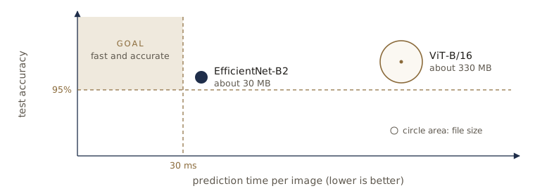
The ViT is slightly more accurate, but it is about eleven times larger and, in this run, more than four times slower. Both clear the accuracy target in the companion chapter’s runs; neither meets the speed target on our slow machine, but EfficientNet-B2 comes far closer. Since we decided to favor speed, we deploy EfficientNet-B2. If later we need more accuracy, the experiment can be rerun with other candidates — deployment decisions are revisited, not made once.
A Gradio demo
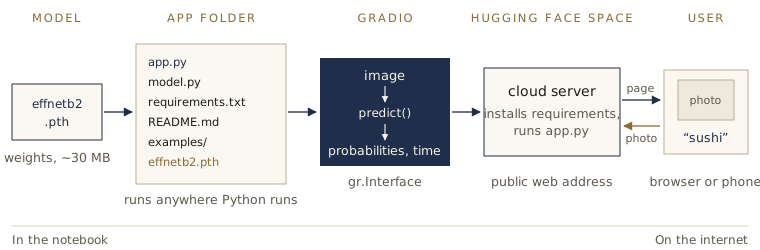
Gradio is a Python library that turns a function into a web page. You describe the inputs (an image upload box), the outputs (a label with probabilities, a number), and the function that maps one to the other; Gradio builds the interface. It is the same inputs → model → outputs picture as always: for FoodVision Mini the input is an image, the function is a predict() that runs our model, and the outputs are the class probabilities and the prediction time.
Install it in Colab, then import it:
!pip install -q gradio
import gradio as gr
print(f"Gradio version: {gr.__version__}")
Gradio version: 6.28.0
The prediction function
Gradio calls our function once for every uploaded photo. It should take an image, prepare it with the model’s transforms, predict, and return two things: a dictionary mapping each class name to its probability (the format Gradio’s Label output expects), and the time the prediction took.
from typing import Tuple

effnetb2.to("cpu")   # the deployed app will run on a CPU

def predict(img) -> Tuple[Dict, float]:
    """Predict the class of a PIL image; return class probabilities and the time taken."""
    start_time = timer()
    img = effnetb2_transforms(img).unsqueeze(0)   # transform and add a batch dimension
    effnetb2.eval()
    with torch.inference_mode():
        pred_probs = torch.softmax(effnetb2(img), dim=1)
    pred_labels_and_probs = {class_names[i]: float(pred_probs[0][i])
                             for i in range(len(class_names))}
    pred_time = round(timer() - start_time, 5)
    return pred_labels_and_probs, pred_time
Try it on one test image:
import random

random.seed(42)
random_image_path = random.choice(test_data_paths)
pred_dict, pred_time = predict(img=Image.open(random_image_path))

print(f"Image: {random_image_path}")
print(f"Classes returned: {list(pred_dict.keys())}")
print(f"Probabilities sum to: {sum(pred_dict.values()):.3f}")
print(f"Prediction time: {pred_time} seconds")
Image: data/pizza_steak_sushi_20_percent/test/pizza/3785667.jpg
Classes returned: ['pizza', 'steak', 'sushi']
Probabilities sum to: 1.000
Prediction time: 0.11121 seconds
The function returns one probability per class, adding up to 1. With the trained model you would print pred_dict itself and typically see most of the probability on the correct class.
Example images
An interface is easier to try if it offers a few example inputs to click. Gradio takes them as a list of lists — one inner list per example, one entry per input:
example_list = [[str(filepath)] for filepath in random.sample(test_data_paths, k=3)]
for example in example_list:
    print(example)
['data/pizza_steak_sushi_20_percent/test/pizza/148765.jpg']
['data/pizza_steak_sushi_20_percent/test/steak/2475366.jpg']
['data/pizza_steak_sushi_20_percent/test/steak/2069289.jpg']
Building the interface
gr.Interface puts the pieces together:
fn— the function to call,predict;inputs—gr.Image(type="pil"), an image upload box that hands our function a PIL image;outputs— one component per returned value:gr.Labelfor the probability dictionary andgr.Numberfor the time;examples,title,description,article— example inputs and text shown above and below the demo.
title = "FoodVision Mini"
description = ("An EfficientNet-B2 feature extractor that classifies photos of food "
               "as pizza, steak, or sushi.")
article = "Built in module 09 of EAS 510, Basics of Artificial Intelligence."

demo = gr.Interface(fn=predict,
                    inputs=gr.Image(type="pil"),
                    outputs=[gr.Label(num_top_classes=3, label="Predictions"),
                             gr.Number(label="Prediction time (s)")],
                    examples=example_list,
                    title=title,
                    description=description,
                    article=article)

print(type(demo).__name__)
print("inputs: ", [type(c).__name__ for c in demo.input_components])
print("outputs:", [type(c).__name__ for c in demo.output_components])
Interface
inputs:  ['Image']
outputs: ['Label', 'Number']
Now start it:
demo.launch(share=True)
In Colab the demo appears inside the notebook, and share=True also prints a temporary public link (Gradio keeps it for at most a week) that you can open on your phone. Upload a photo of food, or click an example, and the predicted probabilities and the time appear on the right. This is the moment to try inputs the model never saw: a burger, a photo of your desk, a blurry picture of sushi.
Turning the demo into an app
The shared link dies when the notebook stops. For a permanent home we package the demo into a folder that can run on its own, anywhere Python runs:
demos/
└── foodvision_mini/
    ├── 09_pretrained_effnetb2_feature_extractor_pizza_steak_sushi_20_percent.pth
    ├── app.py
    ├── model.py
    ├── requirements.txt
    ├── README.md
    └── examples/
        ├── example_1.jpg
        ├── example_2.jpg
        └── example_3.jpg
- the
.pthfile holds the trained weights; model.pyholdscreate_effnetb2_model(), so the app can rebuild the architecture and its transforms;app.pyloads the model, definespredict(), and builds and launches the Gradio interface (Hugging Face Spaces looks for a file with this name);requirements.txtlists the Python packages the app needs;README.mdconfigures the Space and holds the model card (see Using AI responsibly);examples/holds the example images.
The folder, examples, and model file
import shutil

foodvision_mini_demo_path = Path("demos/foodvision_mini")
if foodvision_mini_demo_path.exists():            # start from an empty folder
    shutil.rmtree(foodvision_mini_demo_path)
(foodvision_mini_demo_path / "examples").mkdir(parents=True)

# Copy the three example images into the app folder
for example in example_list:
    source = Path(example[0])
    destination = foodvision_mini_demo_path / "examples" / source.name
    shutil.copy2(src=source, dst=destination)
    print(f"[INFO] Copied {source.name} to {destination}")

# Move the trained model into the app folder
model_destination = foodvision_mini_demo_path / Path(effnetb2_model_path).name
shutil.move(src=effnetb2_model_path, dst=model_destination)
print(f"[INFO] Moved model to {model_destination}")
[INFO] Copied 148765.jpg to demos/foodvision_mini/examples/148765.jpg
[INFO] Copied 2475366.jpg to demos/foodvision_mini/examples/2475366.jpg
[INFO] Copied 2069289.jpg to demos/foodvision_mini/examples/2069289.jpg
[INFO] Moved model to demos/foodvision_mini/09_pretrained_effnetb2_feature_extractor_pizza_steak_sushi_20_percent.pth
model.py
The %%writefile magic from module 05 saves a cell as a file. model.py is the same create_effnetb2_model() as above, with its imports:
%%writefile demos/foodvision_mini/model.py
import torch
import torchvision
from torch import nn


def create_effnetb2_model(num_classes: int = 3, seed: int = 42):
    """Create an EfficientNet-B2 feature extractor and its image transforms."""
    weights = torchvision.models.EfficientNet_B2_Weights.DEFAULT
    transform = weights.transforms()
    model = torchvision.models.efficientnet_b2(weights=weights)

    for param in model.parameters():
        param.requires_grad = False

    torch.manual_seed(seed)
    model.classifier = nn.Sequential(
        nn.Dropout(p=0.3, inplace=True),
        nn.Linear(in_features=1408, out_features=num_classes),
    )
    return model, transform
Writing demos/foodvision_mini/model.py
app.py
app.py has four parts: imports and class names; the model, rebuilt and loaded with the saved weights; the predict() function; and the Gradio interface. Two details differ from the notebook. torch.load(..., map_location=torch.device("cpu")) loads the weights onto the CPU even if they were saved from a GPU — without it, loading a GPU-trained model on a CPU-only server fails. And the examples list is built from whatever is in the examples/ folder.
%%writefile demos/foodvision_mini/app.py
### 1. Imports and class names ###
import os
from timeit import default_timer as timer
from typing import Dict, Tuple

import gradio as gr
import torch

from model import create_effnetb2_model

class_names = ["pizza", "steak", "sushi"]

### 2. Model and transforms ###
effnetb2, effnetb2_transforms = create_effnetb2_model(num_classes=len(class_names))
effnetb2.load_state_dict(
    torch.load(
        f="09_pretrained_effnetb2_feature_extractor_pizza_steak_sushi_20_percent.pth",
        map_location=torch.device("cpu"),   # load onto the CPU
    )
)

### 3. Predict function ###
def predict(img) -> Tuple[Dict, float]:
    """Predict the class of a PIL image; return class probabilities and the time taken."""
    start_time = timer()
    img = effnetb2_transforms(img).unsqueeze(0)
    effnetb2.eval()
    with torch.inference_mode():
        pred_probs = torch.softmax(effnetb2(img), dim=1)
    pred_labels_and_probs = {class_names[i]: float(pred_probs[0][i])
                             for i in range(len(class_names))}
    pred_time = round(timer() - start_time, 5)
    return pred_labels_and_probs, pred_time

### 4. Gradio app ###
title = "FoodVision Mini"
description = ("An EfficientNet-B2 feature extractor that classifies photos of food "
               "as pizza, steak, or sushi.")
article = ("Built in module 09 of EAS 510, Basics of Artificial Intelligence. "
           "See the model card for limitations.")

example_list = [["examples/" + example] for example in sorted(os.listdir("examples"))]

demo = gr.Interface(fn=predict,
                    inputs=gr.Image(type="pil"),
                    outputs=[gr.Label(num_top_classes=3, label="Predictions"),
                             gr.Number(label="Prediction time (s)")],
                    examples=example_list,
                    title=title,
                    description=description,
                    article=article,
                    flagging_mode="never")   # don't store users' images

if __name__ == "__main__":
    demo.launch()
Writing demos/foodvision_mini/app.py
The last two lines launch the demo only when the file is run as a program (python app.py, which is what Hugging Face Spaces does), not when another script imports it. That lets us test the app without starting a web server.
requirements.txt
requirements.txt lists the packages the server must install, one per line. Pin the exact versions you tested with (torch==2.14.0 rather than just torch), so that a future release cannot break the app. Rather than typing them, read them from the running notebook:
requirements = "\n".join([
    f"torch=={torch.__version__.split('+')[0]}",             # drop the "+cu130" build tag
    f"torchvision=={torchvision.__version__.split('+')[0]}",
    f"gradio=={gr.__version__}",
])
(foodvision_mini_demo_path / "requirements.txt").write_text(requirements + "\n")
print(requirements)
torch==2.14.0
torchvision==0.29.0
gradio==6.28.0
Smoke-testing the app
Before uploading anything, check that app.py runs: load it the way Python would, from inside its own folder (it opens files by relative paths such as examples/), and look at what it built.
import importlib
import os
import sys

notebook_dir = os.getcwd()
os.chdir(foodvision_mini_demo_path)   # run from inside the app folder
sys.path.insert(0, os.getcwd())       # so that `import model` and `import app` find its files
try:
    import app
    importlib.reload(app)             # pick up the latest app.py if it was imported before
    print("inputs: ", [type(c).__name__ for c in app.demo.input_components])
    print("outputs:", [type(c).__name__ for c in app.demo.output_components])
    print("examples:", app.example_list)
    probs, seconds = app.predict(Image.open(app.example_list[0][0]))
    print(f"predict() returned {len(probs)} probabilities in {seconds} s")
finally:
    os.chdir(notebook_dir)
    sys.path.pop(0)
inputs:  ['Image']
outputs: ['Label', 'Number']
examples: [['examples/148765.jpg'], ['examples/2069289.jpg'], ['examples/2475366.jpg']]
predict() returned 3 probabilities in 0.12208 s
The app loads the saved weights, finds its examples, and makes a prediction. To try the full app on your own computer, download the folder, and in a terminal:
cd foodvision_mini
python3 -m venv env                  # a fresh, empty Python environment
source env/bin/activate              # on Windows: env\Scripts\activate
pip install -r requirements.txt
python3 app.py                       # then open http://127.0.0.1:7860
In Colab, zip the folder and download it with !cd demos/foodvision_mini && zip -r ../foodvision_mini.zip * followed by from google.colab import files; files.download("demos/foodvision_mini.zip").
Deploying to Hugging Face Spaces
Hugging Face hosts models, datasets, and demo apps; you can think of it as GitHub for machine learning. A Space is a small hosted app: you upload a folder with an app.py, and Hugging Face installs the requirements, runs the app on one of its servers, and gives it a public web address. At the time of writing, a basic CPU machine for a Space costs nothing; check the current plans.
The steps, using the website:
- Create a free account and verify your email.
- Click New Space (from your profile, or huggingface.co/new-space).
- Name it, for example
foodvision_mini; choose a license (MIT is a common choice for course work). - Choose Gradio as the Space SDK and the basic CPU hardware.
- Choose public or private, then Create Space.
- On the Space’s Files tab, choose Add file → Upload files, and upload everything in
demos/foodvision_mini/, keeping theexamples/folder. Replace the automatically createdREADME.mdwith ours. - Watch the Logs: the first build installs the requirements and takes a few minutes. When it finishes, the app appears on the Space’s page at
https://huggingface.co/spaces/<your-username>/foodvision_mini.
You can also upload from Python with the huggingface_hub library. This needs an access token with write permission, created under Settings → Access Tokens on the Hugging Face website:
from huggingface_hub import HfApi, login

login()   # paste your access token when asked; never write it into a notebook you share

api = HfApi()
repo_id = "your-username/foodvision_mini"
api.create_repo(repo_id=repo_id, repo_type="space", space_sdk="gradio", exist_ok=True)
api.upload_folder(folder_path="demos/foodvision_mini", repo_id=repo_id, repo_type="space")
A Space is also a git repository, so you can git clone it and git push your files. With plain git, large files such as our 30 MB model need a large-file extension such as Git LFS (large file storage); the Hugging Face documentation describes the current setup. The web upload and upload_folder handle large files for you.
Note. If the Space shows an error, read the Logs tab from the bottom up. The usual causes are a package missing from
requirements.txt, a file name inapp.pythat doesn’t match the uploaded file, or a model saved from a GPU and loaded withoutmap_location.
Scaling up: FoodVision Big
The same pipeline works for a bigger problem. The full Food-101 dataset has 101 classes of food with 1,000 images each (750 for training and 250 for testing per class). The companion chapter builds FoodVision Big from it. We describe the changes rather than train it, since it needs a GPU and a multi-gigabyte download.
The model is create_effnetb2_model(num_classes=101). Only the head grows — from 3 outputs to 101 — so the model hardly gets bigger:
effnetb2_food101, _ = create_effnetb2_model(num_classes=101)
total = sum(p.numel() for p in effnetb2_food101.parameters())
trainable = sum(p.numel() for p in effnetb2_food101.parameters() if p.requires_grad)
print(f"FoodVision Big: {total:,} parameters, {trainable:,} trainable")
print(f"FoodVision Mini: {effnetb2_total_params:,} parameters, "
      f"{sum(p.numel() for p in effnetb2.parameters() if p.requires_grad):,} trainable")
FoodVision Big: 7,843,303 parameters, 142,309 trainable
FoodVision Mini: 7,705,221 parameters, 4,227 trainable
The head now has \(1408 \times 101 + 101 = 142{,}309\) parameters, but the frozen backbone — almost all of the model — is unchanged, so the saved file grows only slightly. The other changes, sketched in code:
from torchvision import datasets, transforms

# Augment the training images only (module 04); test images get the plain transforms
food101_train_transforms = transforms.Compose([transforms.TrivialAugmentWide(),
                                               effnetb2_transforms])

train_data = datasets.Food101(root="data", split="train",
                              transform=food101_train_transforms, download=True)
test_data = datasets.Food101(root="data", split="test",
                             transform=effnetb2_transforms, download=True)
food101_class_names = train_data.classes

# Train on a random 20% of each split first, to keep experiments quick
train_subset, _ = torch.utils.data.random_split(train_data, [0.2, 0.8],
                                                generator=torch.Generator().manual_seed(42))
test_subset, _ = torch.utils.data.random_split(test_data, [0.2, 0.8],
                                               generator=torch.Generator().manual_seed(42))

# Label smoothing: the target for the true class becomes a little less than 1,
# which discourages over-confident predictions when there are many classes
loss_fn = nn.CrossEntropyLoss(label_smoothing=0.1)
After training for about 5 epochs, the app folder is the same as FoodVision Mini’s, with two differences: model.py is called with num_classes=101, and the 101 class names, too many to type into app.py, are saved to a class_names.txt file that app.py reads at startup.
Using AI responsibly
A public app puts your model in front of people you have never met, using it in ways you did not plan. Before you share the link, work through four questions.
Bias and fairness: whose data?
A model learns from its training data and nothing else, so start by asking where that data came from and who it represents. Food-101 was assembled from photos posted to a food-photo sharing website. Its 101 classes are dishes that were popular on that site, photographed mostly in the style its users favored. That raises concrete questions for FoodVision:
- Which foods are missing? Many cuisines have no class at all. A user whose everyday meals are not among the classes will get wrong answers every time, however well the model scores on its test set.
- Which versions of a food are represented? “Pizza” in the training data may look like one regional style. A home-cooked version, or a different regional one, may be recognized less reliably.
- Which photos? Well-lit restaurant photos on phones of a certain era may not look like a dim kitchen photo on a cheap camera.
An overall test accuracy can hide all of this. Measure accuracy per class (for example effnetb2_test_pred_df.groupby("class_name")["correct"].mean()), and, when you can, test on photos collected from the people who will actually use the app. For FoodVision the harm of a mistake is small. For a model that screens job applications or flags structural defects, the same questions decide who is failed by the system.
Privacy: the images people upload
Every photo sent to a Space travels to the server that runs your app (for a Space, one of Hugging Face’s). Photos can show faces, homes, and documents, and phone photos often carry hidden metadata such as the GPS location where they were taken.
- Keep only what you need. Our
predict()uses the image in memory and discards it. Gradio’s flagging feature, which is on by default, lets users save an input and output to a file on the server; that is whyapp.pysetsflagging_mode="never". If you turn flagging on to collect hard examples, say so on the page. - Say what happens to uploads. One sentence in the description (“Images are processed in memory and not stored”) tells users what to expect.
- Private versus public. A public Space can be used by anyone, and the files in it — including the model — can be downloaded by anyone. Make the Space private if either is a problem.
Security: risks to the model and the app
- Only load model files you trust.
torch.loadreads a format that can, in general, contain code that runs on loading. Recent PyTorch versions load withweights_only=Trueby default, which accepts only tensors and plain data; keep that default, and never load a.pthfile from an unknown source with it turned off. - Keep secrets out of the code. Access tokens and passwords belong in the Space’s Settings → Variables and secrets, read with
os.environ, never inapp.pyor a notebook you share. - Expect unexpected inputs. A public app will receive huge images, non-images, and deliberately strange inputs.
gr.Imageis built for image uploads, but keep the rest of your code tolerant (for example, convert every image to RGB before transforming it). - Know that models can be fooled. Small, carefully chosen changes to an image — adversarial examples — can flip a classifier’s answer. For a food demo this does not matter; for a safety-related model it is a known risk to test for.
- Pin your dependencies, as we did in
requirements.txt, so the app does not change behavior when a package updates.
Explainability: showing what the model is doing
Deep networks do not give reasons for their answers, but an app can still help users judge a prediction:
- Show probabilities, not just a label.
gr.Label(num_top_classes=3)shows all three probabilities, so “pizza 0.51, steak 0.47” reads very differently from “pizza 0.99”. - Admit uncertainty. You can return “not sure” when the top probability falls below a threshold. This helps with photos between classes, but not with the dog photo: a model trained only on three foods can be confidently wrong about something that is none of them. Handling that needs a separate “food or not food” check, or a class for “other”.
- Look inside when it matters. Methods such as Grad-CAM highlight the parts of an image that most influenced a prediction; they can reveal a model that relies on the plate or the background rather than the food.
- Publish the failures you found. Example images where the model is wrong tell users more than an accuracy figure.
A model card
A model card is a short document that ships with a model and says what it is for, how it was trained and tested, and where it fails — a data sheet for a model, in the sense engineers use for materials and components. The idea comes from Mitchell et al., “Model Cards for Model Reporting” (2019), and Hugging Face displays a Space’s README.md on its page, so the README is the natural place for it. On Spaces the README also starts with a short configuration block that tells Hugging Face how to run the app. We write both from Python, so that the Gradio version in the configuration matches requirements.txt:
model_card = f"""---
title: FoodVision Mini
sdk: gradio
sdk_version: {gr.__version__}
app_file: app.py
license: mit
pinned: false
---

# FoodVision Mini

## Model details
- EfficientNet-B2 image classifier (torchvision, pretrained on ImageNet) used as a
  feature extractor: frozen backbone, new 3-class head trained for 10 epochs with PyTorch.
- Author and date: <your name>, <date>. Course project, EAS 510.

## Intended use
- Classify a photo of a single dish as pizza, steak, or sushi, for demonstration and teaching.
- Not intended for dietary, allergy, or medical decisions, or for photos of people.

## Training and evaluation data
- 20% sample of the pizza, steak, and sushi classes of Food-101 (Bossard et al., 2014):
  450 training images and 150 test images, collected from a food-photo sharing website.

## Performance
- Test accuracy on the 150 test images: <your number>.
- Average prediction time on a 1-thread CPU: <your number> seconds.

## Limitations
- Always answers pizza, steak, or sushi, even for photos of other foods or of non-food.
- Trained on few images of one photo style; styles, cuisines, and lighting that differ
  from the training photos may be classified less reliably.
- A high probability is not a guarantee of a correct answer.

## Privacy
- Uploaded images are processed in memory and not stored (flagging is turned off).
"""

(foodvision_mini_demo_path / "README.md").write_text(model_card)
for path in sorted(foodvision_mini_demo_path.iterdir()):
    print(path.name)
09_pretrained_effnetb2_feature_extractor_pizza_steak_sushi_20_percent.pth
README.md
__pycache__
app.py
examples
model.py
requirements.txt
The app folder is complete. (__pycache__ holds Python’s compiled copies of the scripts, created by the smoke test; there is no need to upload it.) Fill in the placeholders with your own measured numbers before you publish — a model card with invented or copied numbers is worse than none.
Habit. Write the model card while you build the model, not after. If you cannot fill in “Intended use” and “Limitations”, you are not ready to deploy.
Summary
| Task | Code or tool |
|---|---|
| Build a candidate with its transforms | create_effnetb2_model(num_classes), create_vit_model(num_classes) → (model, transform) |
| Measure file size | Path(path).stat().st_size / (1024 * 1024) |
| Count parameters | sum(torch.numel(p) for p in model.parameters()) |
| Time predictions like a deployed app | one image at a time, on the CPU, with timeit.default_timer |
| Build a demo | gr.Interface(fn=predict, inputs=gr.Image(type="pil"), outputs=[gr.Label(...), gr.Number(...)]) |
| Run it | demo.launch(share=True) (notebook); python app.py (app folder) |
| Load weights on a CPU server | torch.load(path, map_location=torch.device("cpu")) |
| Publish | Hugging Face Space with app.py, model.py, requirements.txt, README.md, weights, examples/ |
Three ideas to carry forward: decide where and how a model will be used before you choose it, because speed and size matter as much as accuracy once a model leaves the notebook; measure on hardware like the deployed hardware; and document a deployed model truthfully — who it is for, what data it learned from, and where it fails.
Exercises
- Time both models on a Colab GPU (
device="cuda") as well as the CPU, with the trained models. Does the GPU close the gap between the ViT and EfficientNet-B2? What does that suggest about where each model should run? - Try
torch.set_num_threads(2)and(4)(in Colab) and time EfficientNet-B2 again. How does the prediction time change with the number of CPU cores? - Find the “most wrong” predictions of your trained EfficientNet-B2: the wrong predictions with the highest probability. Plot five of them and write one sentence about each: why might the model have been fooled?
- Add a confidence threshold to
predict(): if the top probability is below 0.6, add an entry that tells the user the model is not sure. Upload a photo of a non-food object. Does the threshold catch it? Explain why or why not. - Deploy FoodVision Mini to your own Hugging Face Space, following the steps in this module. Test it on your phone with photos of your own meals, and add three of the model’s failures to the Limitations section of your model card.
- Pick any dataset from
torchvision.datasets, train a feature extractor on it for 5 epochs, and deploy it as a Gradio app with a model card. - Write down three ways the deployed FoodVision Mini could fail in use (not in testing), and a practical fix for each.
- Compute the per-class accuracy of your trained model on the test set. Is one class clearly worse than the others? What data would you collect to fix it?
- In your own words. Take a model from your engineering field (for example, detecting corrosion in inspection photos, or predicting a pump failure from vibration data). Would you deploy it on-device or in the cloud, and online or offline? What latency does the application need? Write three sentences for its model card: intended use, one out-of-scope use, and one limitation.
Going further
- The Gradio documentation — especially the list of input and output components and the
BlocksAPI for more complex layouts. - Hugging Face Spaces documentation, including the configuration reference for the README header.
- Mitchell et al., Model Cards for Model Reporting (2019) — the original proposal, with example cards.
- PyTorch’s tutorial on real-time inference on a Raspberry Pi — deploying a vision model to a small edge computer.
- Google’s People + AI Guidebook — practical guidance on designing AI products that set the right expectations for users.
These notes follow the path of Daniel Bourke's Learn PyTorch for Deep Learning (MIT license), rewritten for engineering students meeting Python and machine learning for the first time.