EAS 510 · Module 07 · Week 8
Experiment Tracking
Running many experiments on purpose — changing one thing at a time, logging results, and choosing a model with evidence.
Companion reading: Learn PyTorch for Deep Learning, chapter 07
By the end of this module you can
- Explain why experiment tracking matters once you train more than a handful of models, and compare the common ways of doing it.
- Log training and test loss and accuracy to TensorBoard with
SummaryWriter, and open the results in Colab or on your own computer. - Write a
create_writer()helper that gives every experiment its own clearly named log folder. - Design a small set of experiments that changes one factor at a time — amount of data, model size, and training length.
- Run a series of experiments in a loop, saving each model, and smoke-test the loop cheaply before the full run.
- Compare the runs, choose a model with evidence, and load it back to make predictions.
Contents
- Why track experiments
- Getting set up
- Getting the data
- Datasets and DataLoaders
- Two feature-extractor models
- Logging one run to TensorBoard
- Viewing results in TensorBoard
- Designing a series of experiments
- Running the experiments
- Comparing the results
- Loading the best model and making predictions
- Summary
- Exercises
- Going further
In module 06 we took a pretrained EfficientNet, froze its backbone, gave it a new classifier head, and trained it to tell pizza, steak, and sushi apart. We will call that classifier FoodVision Mini. We judged it by reading the printed loss and accuracy and by plotting a results dictionary. That works for one or two models. It stops working the moment you start asking “would more data help? a bigger model? longer training?” — because each question means another training run, and soon you have a dozen runs and no reliable record of which was which.
This module is about running experiments on purpose. You will log every run to TensorBoard, give each run a folder whose name says exactly what it was, design a small grid of experiments that changes one thing at a time, run them in a loop, and pick the best model from the evidence rather than from memory. Nothing here makes a model more accurate by itself. What it does is make the question “which change helped?” answerable.
Why track experiments
In machine learning, an experiment is one training run with one particular setup: a dataset, a model, a set of hyperparameters, a number of epochs, a random seed. You change something, train, and see what happened. Deep learning is empirical — there is rarely a formula that tells you in advance whether a change will help — so you learn by running many experiments.
The difficulty is bookkeeping. After ten runs, can you say which one used 20% of the data and the smaller model? Which test accuracy went with which learning rate? If you cannot, the runs were wasted. Experiment tracking is the habit, and the tooling, of recording for every run:
- what you changed — the data, the model, the hyperparameters, the seed;
- what happened — loss and accuracy at every epoch, for training and test data;
- what you got — the saved model file, so the best run can be used later.
If you have worked in a materials or structures lab this will feel familiar. A test program is only useful if each specimen is labeled and each result is written down next to the conditions that produced it. Experiment tracking is the lab notebook for model training.
Ways to track experiments
There are many tools. Four common choices:
| Method | Setup | Strengths | Drawbacks | Cost |
|---|---|---|---|---|
| Python dictionaries, CSV files, printouts | None | Nothing to install; pure Python | Becomes unmanageable beyond a few runs; easy to lose track | Free |
| TensorBoard | Install tensorboard |
Supported directly by PyTorch (torch.utils.tensorboard); widely used; runs locally |
Interface is plainer than the hosted tools; sharing takes extra work | Free |
| Weights & Biases | Install wandb, create an account |
Polished web dashboard; easy to share runs; tracks almost anything | Your logs live on an outside service | Free tier for individuals; check current terms |
| MLflow | Install mlflow |
Fully open source; covers the whole model life cycle; many integrations | Setting up a shared tracking server takes more work | Free |
We use TensorBoard because PyTorch supports it directly, it runs on your own machine or in Colab, and it needs no account. The ideas — one folder or record per run, metrics logged every epoch, runs compared side by side — carry over directly to the other tools.
Getting set up
We reuse the going_modular package from module 05. If you are in a fresh Colab runtime, this cell downloads the reference copy of its scripts:
import requests
from pathlib import Path
Path("going_modular").mkdir(exist_ok=True)
base = "https://raw.githubusercontent.com/mrdbourke/pytorch-deep-learning/main/going_modular/going_modular/"
for name in ["data_setup.py", "engine.py", "model_builder.py", "utils.py"]:
    path = Path("going_modular") / name
    if not path.exists():
        path.write_text(requests.get(base + name).text)
Now the usual imports and device-agnostic setup:
import torch
import torchvision
from torch import nn
from torchvision import transforms

from going_modular import data_setup, engine, utils

device = "cuda" if torch.cuda.is_available() else "cpu"
print(f"torch {torch.__version__}, torchvision {torchvision.__version__}, device: {device}")
torch 2.14.0+cu130, torchvision 0.29.0+cu130, device: cpu
These notes were run on a CPU. Turn on a GPU in Colab (Runtime → Change runtime type) before the training sections; the full set of experiments is slow without one.
A helper to set the seeds
We will set the random seed before every experiment so that each one starts from the same random numbers. Since we will do it often, we wrap it in a function:
def set_seeds(seed: int = 42):
    """Set the random seeds for PyTorch on the CPU and the GPU."""
    torch.manual_seed(seed)       # CPU operations
    torch.cuda.manual_seed(seed)  # GPU operations (ignored if there is no GPU)
Seeds make runs repeatable, which matters when two experiments differ by a percent or two and you want to know whether the difference is real. Outside of teaching and experiments you rarely need them.
Getting the data
We need two versions of the pizza, steak, and sushi images: the 10% subset of the Food-101 dataset we have used so far, and a 20% subset with twice as many training images. Both are zip files. A small function downloads a zip file and unpacks it, skipping the download if the folder is already there:
import io
import zipfile

def download_data(source: str, destination: str) -> Path:
    """Download a zipped dataset from `source` and unzip it into data/<destination>."""
    image_path = Path("data") / destination
    if image_path.is_dir():
        print(f"[INFO] {image_path} already exists, skipping download.")
    else:
        print(f"[INFO] Downloading {Path(source).name} and unzipping to {image_path}...")
        image_path.mkdir(parents=True, exist_ok=True)
        response = requests.get(source)
        with zipfile.ZipFile(io.BytesIO(response.content)) as zip_ref:
            zip_ref.extractall(image_path)
    return image_path

data_url = "https://raw.githubusercontent.com/mrdbourke/pytorch-deep-learning/main/data/"
data_10_percent_path = download_data(source=data_url + "pizza_steak_sushi.zip",
                                     destination="pizza_steak_sushi")
data_20_percent_path = download_data(source=data_url + "pizza_steak_sushi_20_percent.zip",
                                     destination="pizza_steak_sushi_20_percent")
[INFO] Downloading pizza_steak_sushi.zip and unzipping to data/pizza_steak_sushi...
[INFO] Downloading pizza_steak_sushi_20_percent.zip and unzipping to data/pizza_steak_sushi_20_percent...
Both datasets use the standard image-classification layout — a train/ and a test/ folder, each with one subfolder per class. We take the two training folders, but only one test folder, the one from the 10% set, for every experiment:
train_dir_10_percent = data_10_percent_path / "train"
train_dir_20_percent = data_20_percent_path / "train"
test_dir = data_10_percent_path / "test"

for folder in [train_dir_10_percent, train_dir_20_percent, test_dir]:
    print(f"{str(folder):42s} {len(list(folder.glob('*/*.jpg')))} images")
data/pizza_steak_sushi/train               225 images
data/pizza_steak_sushi_20_percent/train    450 images
data/pizza_steak_sushi/test                75 images
The 20% training set has exactly twice as many images. Keeping the test set fixed is essential: if each experiment were scored on different test images, a change in accuracy could come from the test images rather than from the change you made.
Datasets and DataLoaders
Pretrained torchvision models expect images prepared the way their training images were: resized, turned into tensors, and normalized with the mean and standard deviation of the ImageNet dataset, channel by channel. In module 06 we got these transforms automatically from the weights (weights.transforms()). Here we write them by hand, for a reason: we will compare two different models, and their automatic transforms differ (EfficientNet-B2’s use larger images). One shared transform keeps the input identical across experiments, so the model is the only thing that changes.
# ImageNet mean and standard deviation for each color channel (R, G, B)
normalize = transforms.Normalize(mean=[0.485, 0.456, 0.406],
                                 std=[0.229, 0.224, 0.225])

simple_transform = transforms.Compose([
    transforms.Resize((224, 224)),   # 1. resize every image to 224 x 224
    transforms.ToTensor(),           # 2. turn it into a tensor with values in [0, 1]
    normalize,                       # 3. shift and scale to match ImageNet
])
Now two sets of DataLoaders with data_setup.create_dataloaders() from module 05 — one per training set, sharing the test data:
BATCH_SIZE = 32

train_dataloader_10_percent, test_dataloader, class_names = data_setup.create_dataloaders(
    train_dir=train_dir_10_percent, test_dir=test_dir,
    transform=simple_transform, batch_size=BATCH_SIZE)

train_dataloader_20_percent, test_dataloader, class_names = data_setup.create_dataloaders(
    train_dir=train_dir_20_percent, test_dir=test_dir,
    transform=simple_transform, batch_size=BATCH_SIZE)

print(f"Batches of {BATCH_SIZE} in the 10% training data: {len(train_dataloader_10_percent)}")
print(f"Batches of {BATCH_SIZE} in the 20% training data: {len(train_dataloader_20_percent)}")
print(f"Batches of {BATCH_SIZE} in the test data:          {len(test_dataloader)}")
print(f"Classes: {class_names}")
Batches of 32 in the 10% training data: 8
Batches of 32 in the 20% training data: 15
Batches of 32 in the test data:          3
Classes: ['pizza', 'steak', 'sushi']
Two feature-extractor models
We will compare two sizes of the same model family: EfficientNet-B0 (the one from module 06) and EfficientNet-B2, a larger version with more layers and more parameters. Both become feature extractors in the way you already know: freeze the pretrained backbone (features), and replace the classifier head with a new layer that has one output per class.
The only new thing is the size of that head’s input. The backbone turns each image into a vector of features, and the new nn.Linear layer must accept a vector of that length. For EfficientNet-B0 it is 1280. Rather than guess for B2, look at the classifier of a freshly created model:
effnetb2_weights = torchvision.models.EfficientNet_B2_Weights.DEFAULT
effnetb2 = torchvision.models.efficientnet_b2(weights=effnetb2_weights)
effnetb2.classifier
Sequential(
  (0): Dropout(p=0.3, inplace=True)
  (1): Linear(in_features=1408, out_features=1000, bias=True)
)
EfficientNet-B2 produces 1408 features, and its original head has 1000 outputs (the ImageNet classes) and a dropout rate of 0.3. We keep the dropout and the input size, and change the output size to 3.
Habit. Whenever you pick up a model you have not used before, print its last layer (or run
torchinfo.summary) before you change anything. The input and output shapes tell you what the new head must look like.
Every experiment needs a fresh, untrained head, so we write one function per model. Each function freezes the backbone, sets the seed before creating the new layer (so both models’ heads start from repeatable random numbers), and attaches a name we can use in file and folder names:
OUT_FEATURES = len(class_names)   # 3: pizza, steak, sushi

def create_effnetb0():
    """EfficientNet-B0 feature extractor for pizza, steak, and sushi."""
    weights = torchvision.models.EfficientNet_B0_Weights.DEFAULT
    model = torchvision.models.efficientnet_b0(weights=weights).to(device)
    for param in model.features.parameters():   # 1. freeze the pretrained backbone
        param.requires_grad = False
    set_seeds()                                  # 2. repeatable random head
    model.classifier = nn.Sequential(            # 3. new head: 1280 features -> 3 classes
        nn.Dropout(p=0.2),
        nn.Linear(in_features=1280, out_features=OUT_FEATURES),
    ).to(device)
    model.name = "effnetb0"                      # 4. a name for logs and files
    print(f"[INFO] Created new {model.name} model.")
    return model

def create_effnetb2():
    """EfficientNet-B2 feature extractor for pizza, steak, and sushi."""
    weights = torchvision.models.EfficientNet_B2_Weights.DEFAULT
    model = torchvision.models.efficientnet_b2(weights=weights).to(device)
    for param in model.features.parameters():
        param.requires_grad = False
    set_seeds()
    model.classifier = nn.Sequential(            # new head: 1408 features -> 3 classes
        nn.Dropout(p=0.3),
        nn.Linear(in_features=1408, out_features=OUT_FEATURES),
    ).to(device)
    model.name = "effnetb2"
    print(f"[INFO] Created new {model.name} model.")
    return model
Let’s create one of each and count their parameters — all of them, and just the ones that will be trained:
def count_parameters(model):
    total = sum(p.numel() for p in model.parameters())
    trainable = sum(p.numel() for p in model.parameters() if p.requires_grad)
    return total, trainable

effnetb0 = create_effnetb0()
effnetb2 = create_effnetb2()
for model in [effnetb0, effnetb2]:
    total, trainable = count_parameters(model)
    print(f"{model.name}: {total:>10,} parameters, {trainable:>6,} trainable")
[INFO] Created new effnetb0 model.
[INFO] Created new effnetb2 model.
effnetb0:  4,011,391 parameters,  3,843 trainable
effnetb2:  7,705,221 parameters,  4,227 trainable
EfficientNet-B2 has nearly twice as many parameters in its frozen backbone, which gives it more capacity to represent the images. The trainable parts — the two heads — are almost the same size: \(1280 \times 3 + 3 = 3843\) and \(1408 \times 3 + 3 = 4227\) numbers. Whether the bigger backbone helps is exactly the kind of question an experiment answers.
Logging one run to TensorBoard
The SummaryWriter class
PyTorch talks to TensorBoard through one class, torch.utils.tensorboard.SummaryWriter. A writer saves whatever you give it to event files in a folder called its log directory (log_dir). TensorBoard later reads every event file under a folder and draws charts from them. The main methods:
| Method | What it records |
|---|---|
writer.add_scalar(tag, value, step) |
One number at one step, e.g. the test loss after epoch 3 |
writer.add_scalars(main_tag, {name: value, ...}, step) |
Several numbers on one chart, e.g. training and test loss together |
writer.add_graph(model, example_input) |
The model’s structure, as a clickable diagram |
writer.add_image, add_figure, add_histogram |
Images, matplotlib figures, and distributions of values |
writer.close() |
Writes anything still in memory to disk |
If you create SummaryWriter() with no arguments, it logs to runs/<date-and-time>_<computer name>. That name tells you when a run happened but not what it was. So instead we build the folder name from the things that define an experiment.
A writer per experiment
create_writer() builds a log directory of the form runs/<date>/<experiment name>/<model name>/<extra> and returns a writer pointing at it:
import os
from datetime import datetime
from torch.utils.tensorboard import SummaryWriter

def create_writer(experiment_name: str,
                  model_name: str,
                  extra: str = None) -> SummaryWriter:
    """Create a SummaryWriter logging to runs/<date>/<experiment>/<model>/<extra>."""
    timestamp = datetime.now().strftime("%Y-%m-%d")   # today's date, e.g. 2026-09-28
    if extra:
        log_dir = os.path.join("runs", timestamp, experiment_name, model_name, extra)
    else:
        log_dir = os.path.join("runs", timestamp, experiment_name, model_name)
    print(f"[INFO] Created SummaryWriter, saving to: {log_dir}")
    return SummaryWriter(log_dir=log_dir)
example_writer = create_writer(experiment_name="data_10_percent",
                               model_name="effnetb0",
                               extra="5_epochs")
[INFO] Created SummaryWriter, saving to: runs/2026-09-28/data_10_percent/effnetb0/5_epochs
Everything run on the same day lands under the same date folder, and inside it the path reads like a sentence: 10% of the data, EfficientNet-B0, 5 epochs. You could add the time, the learning rate, or anything else that varies — the folder name is yours to design.
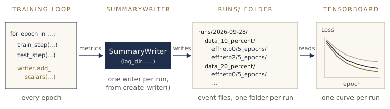
SummaryWriter; the writer appends them to event files in its own folder under runs/; TensorBoard reads every folder under runs/ and overlays the runs so you can compare them.A train() function that logs
We take the train() function from going_modular/engine.py and add an optional writer argument. If a writer is given, the function records the model graph once at the start, logs the losses and accuracies after every epoch, and closes the writer at the end. If not, it behaves exactly as before.
from typing import Dict, List

def train(model: torch.nn.Module,
          train_dataloader: torch.utils.data.DataLoader,
          test_dataloader: torch.utils.data.DataLoader,
          optimizer: torch.optim.Optimizer,
          loss_fn: torch.nn.Module,
          epochs: int,
          device: torch.device,
          writer: SummaryWriter = None) -> Dict[str, List]:
    """Train and test a model, logging the results to `writer` if one is given."""
    results = {"train_loss": [], "train_acc": [], "test_loss": [], "test_acc": []}
    model.to(device)

    # New: record the model's structure once, from one example image
    if writer:
        model.eval()   # trace in eval mode; train_step switches back to train mode
        example_image = torch.randn(1, 3, 224, 224).to(device)
        writer.add_graph(model=model, input_to_model=example_image)

    for epoch in range(epochs):
        train_loss, train_acc = engine.train_step(model=model, dataloader=train_dataloader,
                                                  loss_fn=loss_fn, optimizer=optimizer,
                                                  device=device)
        test_loss, test_acc = engine.test_step(model=model, dataloader=test_dataloader,
                                               loss_fn=loss_fn, device=device)
        print(f"Epoch: {epoch+1} | "
              f"train_loss: {train_loss:.4f} | train_acc: {train_acc:.4f} | "
              f"test_loss: {test_loss:.4f} | test_acc: {test_acc:.4f}")

        results["train_loss"].append(train_loss)
        results["train_acc"].append(train_acc)
        results["test_loss"].append(test_loss)
        results["test_acc"].append(test_acc)

        # New: log this epoch's numbers, two lines per chart
        if writer:
            writer.add_scalars(main_tag="Loss",
                               tag_scalar_dict={"train_loss": train_loss,
                                                "test_loss": test_loss},
                               global_step=epoch)
            writer.add_scalars(main_tag="Accuracy",
                               tag_scalar_dict={"train_acc": train_acc,
                                                "test_acc": test_acc},
                               global_step=epoch)

    # New: make sure everything is written to disk
    if writer:
        writer.close()
    return results
Three details. main_tag names the chart (“Loss”), and the dictionary keys name the lines on it. global_step is the position along the chart’s horizontal axis — here, the epoch number. And the training step itself is unchanged: forward pass, loss, optimizer.zero_grad(), loss.backward(), optimizer.step() all still happen inside engine.train_step.
Train and log one model
Now train one EfficientNet-B0 for 5 epochs on the 10% data, logging to the folder we created above:
model = create_effnetb0()
loss_fn = nn.CrossEntropyLoss()
optimizer = torch.optim.Adam(params=model.parameters(), lr=0.001)

set_seeds()
results = train(model=model,
                train_dataloader=train_dataloader_10_percent,
                test_dataloader=test_dataloader,
                optimizer=optimizer,
                loss_fn=loss_fn,
                epochs=5,
                device=device,
                writer=example_writer)
On a Colab GPU this takes well under a minute. The printed lines look like module 06’s: training and test loss typically fall over the five epochs, and test accuracy climbs well above chance (33% for three classes). The difference is that the same numbers are now also on disk, in runs/2026-09-28/data_10_percent/effnetb0/5_epochs/ (with your date), where they will still be after the notebook is closed.
Viewing results in TensorBoard
TensorBoard is a small web application that reads the runs/ folder and draws charts. How you open it depends on where you work:
| Where you work | How to open TensorBoard |
|---|---|
| Google Colab or Jupyter | Run %load_ext tensorboard, then %tensorboard --logdir runs in a cell. TensorBoard appears inside the notebook. |
| Your own computer (terminal) | Run tensorboard --logdir runs in the folder that contains runs/, then open http://localhost:6006 in a browser. |
| VS Code | Open the Command Palette and run Python: Launch TensorBoard. |
In Colab:
%load_ext tensorboard
%tensorboard --logdir runs
On your own computer, with tensorboard installed (pip install tensorboard):
tensorboard --logdir runs
The Scalars tab shows one chart per main_tag — Loss and Accuracy — with training and test curves on each. Hovering shows the exact value at each step, and the checkboxes on the left switch individual runs on and off. The Graphs tab shows the diagram recorded by add_graph; double-click a block to open it up. Behind the scenes, add_scalars stores each line in its own subfolder (Loss_train_loss, Loss_test_loss, …), which is why TensorBoard’s run list is longer than the number of experiments.
Note. The notebook cells above keep TensorBoard running in the background. If the charts do not update after a new run, click the refresh icon at the top right of TensorBoard, or run the
%tensorboardcell again.
Designing a series of experiments
With one run logged, we can think about many. What could we change? Almost any choice you made while building the model is a candidate:
- the amount of data (and its quality);
- the model — a different architecture, or a bigger or smaller one;
- the training length (number of epochs);
- the learning rate, the optimizer, the batch size;
- data augmentation (module 04);
- the number of layers or hidden units, for models you build yourself.
You cannot test everything, so two rules of thumb help.
Start small, then scale up. Your first experiments should take seconds to minutes. The faster an experiment runs, the more of them you can do, and the sooner you find out what does not work. When something works, then spend more compute on it. (Rich Sutton’s short essay The Bitter Lesson argues that, over the history of AI, methods that make good use of more data and computation have tended to win — a reason to expect bigger models and more data to help, and a reason to check.)
Change one thing at a time. If you switch to a bigger model and double the data in the same run, and accuracy improves, you cannot say which change did it. This is the same principle as holding all but one variable fixed in a lab test. When you want to study several factors, test every combination of them — a full factorial design — so each factor’s effect can be seen with the others held fixed.
For FoodVision Mini our goal is higher test accuracy without the model growing much. We study three factors at two levels each:
- Data: 10% or 20% of the pizza, steak, and sushi images.
- Model: EfficientNet-B0 or EfficientNet-B2.
- Training length: 5 or 10 epochs.
Every combination gives \(2 \times 2 \times 2 = 8\) experiments:
| Experiment | Training data | Model | Epochs |
|---|---|---|---|
| 1 | 10% | EfficientNet-B0 | 5 |
| 2 | 10% | EfficientNet-B2 | 5 |
| 3 | 10% | EfficientNet-B0 | 10 |
| 4 | 10% | EfficientNet-B2 | 10 |
| 5 | 20% | EfficientNet-B0 | 5 |
| 6 | 20% | EfficientNet-B2 | 5 |
| 7 | 20% | EfficientNet-B0 | 10 |
| 8 | 20% | EfficientNet-B2 | 10 |
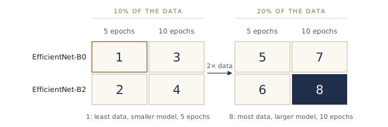
Everything else stays fixed across the eight runs: the test set, the image transform, the optimizer (Adam, learning rate 0.001), the loss function, and the random seed. Each run also starts from a freshly created model, so no experiment inherits training from the one before it.
Running the experiments
Put the levels of each factor into Python lists and a dictionary:
num_epochs = [5, 10]
models = ["effnetb0", "effnetb2"]
train_dataloaders = {"data_10_percent": train_dataloader_10_percent,
                     "data_20_percent": train_dataloader_20_percent}
Next, one function that runs one experiment from start to finish: build a fresh model, a loss function, and an optimizer; create a writer whose folder names the experiment; train; and save the trained model with a file name that also names the experiment.
def run_experiment(dataloader_name: str, model_name: str, epochs: int) -> Dict[str, List]:
    """Train one fresh model on one training set, log it, and save it."""
    # 1. A brand-new model every time, so experiments don't share training
    model = create_effnetb0() if model_name == "effnetb0" else create_effnetb2()

    # 2. A new loss function and optimizer for the new model
    loss_fn = nn.CrossEntropyLoss()
    optimizer = torch.optim.Adam(params=model.parameters(), lr=0.001)

    # 3. Train, logging to runs/<date>/<data>/<model>/<epochs>
    results = train(model=model,
                    train_dataloader=train_dataloaders[dataloader_name],
                    test_dataloader=test_dataloader,
                    optimizer=optimizer,
                    loss_fn=loss_fn,
                    epochs=epochs,
                    device=device,
                    writer=create_writer(experiment_name=dataloader_name,
                                         model_name=model_name,
                                         extra=f"{epochs}_epochs"))

    # 4. Save the trained model so the best one can be reloaded later
    utils.save_model(model=model, target_dir="models",
                     model_name=f"07_{model_name}_{dataloader_name}_{epochs}_epochs.pth")
    return results
Smoke-test first
Before you start eight training runs, run the smallest possible one to make sure the whole pipeline works end to end — data, model, logging, saving. Engineers call this a smoke test: switch it on and see whether anything catches fire. One epoch on the 10% data with the small model is enough:
set_seeds(42)
smoke_results = run_experiment(dataloader_name="data_10_percent",
                               model_name="effnetb0",
                               epochs=1)
It prints the “created” messages, one epoch line, and the path of the saved model. If it runs without an error, the full loop will too — a typo in the saving code is much cheaper to find after one epoch than after the eighth experiment. Let’s check what it left on disk:
for path in sorted(Path("runs").rglob("*")):
    if path.is_dir():
        print(path)
print()
print(sorted(p.name for p in Path("models").glob("*.pth")))
runs/2026-09-28
runs/2026-09-28/data_10_percent
runs/2026-09-28/data_10_percent/effnetb0
runs/2026-09-28/data_10_percent/effnetb0/1_epochs
runs/2026-09-28/data_10_percent/effnetb0/1_epochs/Accuracy_test_acc
runs/2026-09-28/data_10_percent/effnetb0/1_epochs/Accuracy_train_acc
runs/2026-09-28/data_10_percent/effnetb0/1_epochs/Loss_test_loss
runs/2026-09-28/data_10_percent/effnetb0/1_epochs/Loss_train_loss
runs/2026-09-28/data_10_percent/effnetb0/5_epochs

['07_effnetb0_data_10_percent_1_epochs.pth']
Each run has its own folder, with one subfolder per logged line, and the model file’s name says exactly how it was made. (The 5_epochs folder was created along with example_writer. It holds no metrics here because these notes skipped the five-epoch training run; in your notebook it holds that run’s logs.) You can delete the smoke-test folder and file before the real run so they don’t clutter TensorBoard.
The full loop
Now the eight experiments: three nested loops, one per factor, calling run_experiment for each combination. We also keep a small summary of each run’s final test numbers, which will make the comparison easier.
import pandas as pd

set_seeds(42)
summary_rows = []
experiment_number = 0

for dataloader_name in train_dataloaders:           # 10% data, then 20%
    for epochs in num_epochs:                        # 5 epochs, then 10
        for model_name in models:                    # EfficientNet-B0, then B2
            experiment_number += 1
            print(f"[INFO] Experiment {experiment_number}: {model_name}, "
                  f"{dataloader_name}, {epochs} epochs")
            results = run_experiment(dataloader_name, model_name, epochs)
            summary_rows.append({"experiment": experiment_number,
                                 "data": dataloader_name,
                                 "model": model_name,
                                 "epochs": epochs,
                                 "test_loss": results["test_loss"][-1],
                                 "test_acc": results["test_acc"][-1]})
            print("-" * 60)
The order of the loops sets the order of the experiments, and it matches the numbering in the table. On a Colab GPU expect the whole loop to take several minutes or more, most of it in the 10-epoch runs of EfficientNet-B2 on the 20% data. On a CPU it is far slower, which is why these notes show the code without its output.
Watch out. Always create a new model inside the loop. If you created the model once outside it, experiment 2 would continue training the model left over from experiment 1, and every comparison after that would be meaningless.
Comparing the results
Open TensorBoard again (%tensorboard --logdir runs). All eight runs now appear together, each named by its folder path. A few ways to read them:
- Start with the test loss chart. It is usually a smoother signal than accuracy. Find the curve that ends lowest.
- Use the run filter. Typing
effnetb2in the filter box shows only the B2 runs;20_percentshows only the runs with more data. Comparing the filtered sets is a quick way to see one factor at a time. - Look at the gap between training and test curves. A training loss that keeps falling while the test loss flattens or rises is the overfitting you met in module 04.
- Ask what each gain costs. A bigger model and longer training cost time and memory, both when training and when making predictions.
The summary rows from the loop give the same final numbers as a table you can sort:
results_df = pd.DataFrame(summary_rows)
results_df.sort_values("test_acc", ascending=False)
What should you expect? A reasonable hypothesis going in is that more data and a bigger pretrained model will help more than extra epochs, and that the best few runs will be close to each other — which is exactly why you log everything instead of trusting memory. Check whether your own results support that hypothesis. Your numbers will differ somewhat with different hardware and library versions; what matters is the trend, and that you can point to the logs that show it.
Watch out. Our test set has 75 images, so one image is worth roughly \(100 / 75 \approx 1.3\) percentage points of accuracy (a little more for images in the last, smaller batch, because
engine.pyaverages accuracy batch by batch). Two runs that differ by one or two percent may differ by one image, which is within the noise of a different random seed. Before trusting a small difference, repeat both runs with two or three different seeds and compare the averages.
Loading the best model and making predictions
Suppose the evidence points to experiment 8: EfficientNet-B2, 20% of the data, 10 epochs. The loop saved its weights as models/07_effnetb2_data_20_percent_10_epochs.pth. To use it, create a fresh model of the same architecture and load the saved state_dict into it:
best_model_path = "models/07_effnetb2_data_20_percent_10_epochs.pth"

best_model = create_effnetb2()
best_model.load_state_dict(torch.load(best_model_path))
[INFO] Created new effnetb2 model.
<All keys matched successfully>
“All keys matched” means every tensor in the file found a place in the new model — the architecture in create_effnetb2() matches the one that was saved. While we are here, check the file size. It will matter in module 09, when we put a model into an app:
best_model_size = Path(best_model_path).stat().st_size / (1024 * 1024)
print(f"EfficientNet-B2 feature extractor size: {best_model_size:.1f} MB")
EfficientNet-B2 feature extractor size: 29.8 MB
The file holds every parameter, frozen or not, as 32-bit numbers (4 bytes each). About 7.7 million parameters at 4 bytes is roughly 30 MB — and the size does not depend on how well the model was trained.
Predicting on test images
A test-set accuracy is a single number. Looking at individual predictions shows you how the model succeeds and fails. This function opens an image, applies the same transform used in training, and plots the image with the predicted class and its probability:
import matplotlib.pyplot as plt
from PIL import Image

def pred_and_plot_image(model, image_path, class_names,
                        transform=simple_transform, device=device):
    """Predict the class of one image and plot it with the prediction as the title."""
    image = Image.open(image_path).convert("RGB")
    image_tensor = transform(image).unsqueeze(dim=0).to(device)   # add a batch dimension
    model.to(device)
    model.eval()
    with torch.inference_mode():
        probs = torch.softmax(model(image_tensor), dim=1)
    label = probs.argmax(dim=1).item()
    plt.figure()
    plt.imshow(image)
    plt.title(f"Pred: {class_names[label]} | Prob: {probs.max().item():.3f}")
    plt.axis(False)
    plt.show()
Now three random images from the 20% test set — images none of our models trained on:
import random

random.seed(42)
test_image_paths = list((data_20_percent_path / "test").glob("*/*.jpg"))
for image_path in random.sample(test_image_paths, k=3):
    pred_and_plot_image(model=best_model, image_path=image_path, class_names=class_names)
With the trained experiment-8 model you should see mostly correct labels, often with high probabilities. Run the cell a few times to see different images; when a prediction is wrong, look at the photo and ask whether a person could have been confused too.
Predicting on your own image
Finally, an image from outside the dataset. Any photo of pizza, steak, or sushi works; here we download one from the course repository:
custom_image_path = Path("data/04-pizza-dad.jpeg")
if not custom_image_path.is_file():
    image_url = "https://raw.githubusercontent.com/mrdbourke/pytorch-deep-learning/main/images/04-pizza-dad.jpeg"
    custom_image_path.write_bytes(requests.get(image_url).content)

pred_and_plot_image(model=best_model, image_path=custom_image_path, class_names=class_names)
The trained model should label this photo as pizza. Try photos of your own, including ones that are hard (a sushi plate with steak on the side) or out of scope (a salad). The model has only three classes, so it will call a salad one of them, often with high confidence — a limitation we come back to in module 09.
Summary
| Task | Code |
|---|---|
| Make results repeatable | set_seeds(42) → torch.manual_seed, torch.cuda.manual_seed |
| Create a logger | SummaryWriter(log_dir=...), or create_writer(experiment_name, model_name, extra) |
| Log numbers each epoch | writer.add_scalars("Loss", {"train_loss": ..., "test_loss": ...}, global_step=epoch) |
| Log the model structure | writer.add_graph(model, example_input) |
| Finish logging | writer.close() |
| View the logs | %load_ext tensorboard, %tensorboard --logdir runs (Colab); tensorboard --logdir runs (terminal) |
| Run a grid of experiments | nested for loops over the factor levels, a fresh model in each |
| Save and reload the best model | utils.save_model(...); model.load_state_dict(torch.load(path)) |
Three ideas to carry forward: an experiment you did not record is an experiment you did not run; change one thing at a time, and keep the test set fixed, so each difference has a cause; and start small — run a cheap smoke test and a few quick experiments before spending compute on the big ones.
Exercises
Use a Colab GPU for these; exercises 1–4 each add a few training runs.
- Add a third model to the experiment list, such as EfficientNet-B3 (
torchvision.models.efficientnet_b3). Find the size of its classifier’s input by printingmodel.classifier, writecreate_effnetb3(), and compare it with B0 and B2 in TensorBoard. - Add data augmentation as a factor: build a training transform with
transforms.TrivialAugmentWide()(training data only — never augment the test set) and compare EfficientNet-B2 on the 20% data with and without it. You will need a version ofcreate_dataloadersthat takes separate training and test transforms. - Make the learning rate a factor: run EfficientNet-B0 on the 10% data for 5 epochs with learning rates 0.01, 0.001, and 0.0001. Add the learning rate to the log folder name. Which rate trains fastest, and which ends best?
- Repeat experiments 6 and 8 with seeds 0, 1, and 2. Average the final test accuracies for each. Is the difference between 5 and 10 epochs larger than the spread between seeds?
- Extend
train()so that, at the end of training, it logs a figure withwriter.add_figure()— for example, a matplotlib plot of three test images with their predictions. - Load the TensorBoard logs back into Python. Hint:
from tensorboard.backend.event_processing.event_accumulator import EventAccumulator; call.Reload()and.Scalars(tag)on a run folder. Build a pandas DataFrame of the final test loss of every run and sort it. - Try one of the hosted trackers. Sign up for Weights & Biases or install MLflow, and log one experiment from this module with it. What does it record that TensorBoard did not?
- The eight experiments are a full factorial design. How many runs would a full factorial design need for 4 factors at 3 levels each? Suggest how you would cut that number down if each run took an hour.
- In your own words. Pick a model you might build in your engineering field (for example, predicting a material’s strength from its composition, or detecting faults from vibration data). List three factors you would vary, two levels for each, what you would hold fixed, and which single number you would use to choose the winner.
Going further
- PyTorch’s
torch.utils.tensorboarddocumentation lists everySummaryWritermethod. - The PyTorch tutorial Visualizing models, data, and training with TensorBoard logs images, a model graph, and precision–recall curves.
- Rich Sutton, The Bitter Lesson — a two-page essay on why scale has mattered so much in AI.
- Made With ML’s lesson on experiment tracking walks through the same ideas with MLflow.
- The Weights & Biases quickstart shows how to log a PyTorch training loop to a hosted dashboard.
These notes follow the path of Daniel Bourke's Learn PyTorch for Deep Learning (MIT license), rewritten for engineering students meeting Python and machine learning for the first time.