Mathematics of AI · · 26 min read
Probability, likelihood, and where loss functions come from
Why a model should describe a distribution rather than a single answer, how likelihood turns that distribution into a score for the parameters, and how maximizing it produces the loss you train with.
Contents
- Why a model should speak probability
- Random variables and distributions
- Likelihood: the same formula, read the other way
- Independence, products, and why we take logs
- Maximum likelihood
- From likelihood to loss
- Summary
- Exercises
- Going further
A question I hear every semester, usually a few weeks into a machine learning course: why do we train regression models with mean squared error and classifiers with cross-entropy? The common answers are “that’s the convention” and “it works better”. Both are true, and neither explains anything.
The real answer is that the two losses are the same recipe applied to two different assumptions about the data. The recipe is maximum likelihood: write down a probability model for the target, ask which parameters make the observed data most probable, and take the negative logarithm. Assume Gaussian noise on a number and you get squared error. Assume a biased coin for a label and you get cross-entropy. Once you see the recipe, the choice of loss stops being folklore and becomes a modeling decision you can reason about, and change when the assumption is wrong.
This series builds that recipe in three parts. This first part sets up the probability we need: distributions, Bayes’ theorem, likelihood, and maximum likelihood. Part 2 (coming soon) derives mean squared error and shows what happens when its assumption fails. Part 3 (coming soon) derives cross-entropy and explains why squared error is a poor substitute for it.About the code. All code is NumPy, with SciPy for one check, and every printed number on this page comes from running the cells in order.
Laid out step by step, the recipe is a pipeline that every trained model goes through. We are given examples. We choose a model: a distribution with parameters we do not know yet. We score candidate parameters by how well they explain the examples, turn that score into a loss, and train by finding the parameters with the lowest loss. Then the trained model makes predictions. The bottom line of each box follows the running example of this part, a coin tossed 10 times.
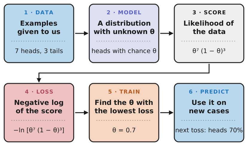
Each section below starts by marking where we are in the pipeline, the way a lecture keeps coming back to its roadmap.
Why a model should speak probability

The examples are given to us, so the first real decision is step 2: what should the model output? Take a model that predicts the sale price of a house from its size, age, and location. Two houses with identical features can still sell for different prices, so no function of the recorded features can predict the price exactly: the features do not determine it.Why not? The buyers differ, the timing differs, one kitchen was redone and the data does not record it.
So the honest output of the model is not one number but a description of the spread of likely prices for those features: a conditional distribution \(p(t \mid \mathbf{x})\) over the target \(t\) given the input \(\mathbf{x}\). A point prediction is a summary of that distribution, such as its mean or its median. Which summary you should report, and which loss trains a model to report it, both follow from what you assume about the spread.
Classification works the same way. An email with a given set of words is spam some of the time, not always. A useful classifier says “spam with probability 0.93”, and that number is again a statement about a distribution, this time over two outcomes.
Training, in this view, means adjusting the model until the distribution it describes agrees with the data. To make “agrees with the data” precise we need a few definitions.
Random variables and distributions
A random variable is a quantity whose value we are uncertain about: the outcome of a coin toss, tomorrow’s closing price, the label of an image. Its distribution says how probable each value is. Random variables come in two kinds, discrete and continuous, and the kind decides how we describe the distribution.Discrete. Values you can list one by one, with gaps in between: heads or tails, the number of heads in 10 tosses (0, 1, …, 10), the class of an image (cat, dog, ship), the next word a language model writes.Continuous. Any value in an interval: a person’s height, tomorrow’s noon temperature, a stock’s one-day return. Between any two possible values there are infinitely many others.
Labels are always discrete, which is why classification and regression end up with different losses in Parts 2 and 3. Some quantities sit in between, as the middle row of the figure shows.In between. A closing price is quoted in cents and an image’s pixels take only 256 brightness levels, so strictly both are discrete, but their steps are so fine that we model them as continuous.
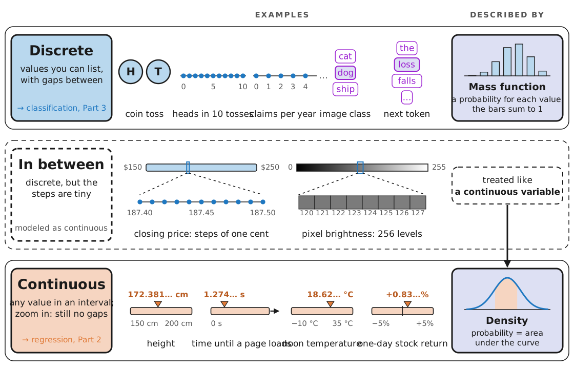
For a discrete variable the distribution is a probability mass function: a list of probabilities \(p(t)\), one per value, each between 0 and 1 and summing to 1. For a continuous variable it is a probability density \(p(t)\): a non-negative function whose integral over the whole line is 1. Probabilities of a continuous variable are areas under the density,
\[P(a \le t \le b) = \int_a^b p(t)\, dt,\]and the probability of any single exact value is zero.Why zero? A single point has no width, so the area above it is zero. Only intervals get probability.
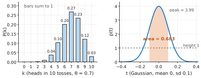
To read the left panel, take a bar’s height as a probability: the bar at 7 says that seven heads has probability 0.27. For an event that covers several values, add their bars: at least eight heads has probability \(0.23 + 0.12 + 0.03 \approx 0.38\).
The right panel cannot be read that way. Its height reaches 3.99, more than any probability can be. Read areas instead: the shaded area says that \(t\) falls between \(-0.1\) and \(0.1\) with probability 0.683, and the whole area under the curve is 1. A quick check of the height and the total area:Keep in mind. The likelihoods we compute for continuous targets are products of densities, so they are not probabilities either. Only comparisons between parameter values matter.
import numpy as np
from scipy.optimize import minimize

np.set_printoptions(precision=4, suppress=True)
rng = np.random.default_rng(2026)

def gauss_pdf(t, mu, sigma):
    """Density of a Gaussian with mean mu and standard deviation sigma."""
    return np.exp(-0.5 * ((t - mu) / sigma) ** 2) / (sigma * np.sqrt(2 * np.pi))

grid = np.linspace(-1, 1, 200_001)
dens = gauss_pdf(grid, 0.0, 0.1)
print(f"peak density      : {dens.max():.4f}")
print(f"area under curve  : {np.trapezoid(dens, grid):.6f}")
peak density      : 3.9894
area under curve  : 1.000000
The sum and product rules
So far each distribution has described a single quantity. A model always deals with at least two at once, an input and a target: the words in an email and whether it is spam, a house’s features and its price. Two rules govern how their probabilities fit together, and all the probability theory we need rests on them. For two random variables \(X\) and \(Y\):
Definition. The sum rule recovers the distribution of one variable by adding up the joint distribution over the other, and the product rule splits a joint distribution into a marginal and a conditional:
\[p(X) = \sum_{Y} p(X, Y), \qquad p(X, Y) = p(Y \mid X)\, p(X).\]For continuous variables the sum becomes an integral.
Here \(p(X, Y)\) is the joint distribution, \(p(X)\) the marginal, and \(p(Y \mid X)\) the conditional distribution of \(Y\) once \(X\) is known. Two variables are independent when \(p(X, Y) = p(X)\, p(Y)\): knowing one tells you nothing about the other.
A small example. Take 100 emails and record two things about each: whether it contains the word “free” (\(X\)) and whether it is spam (\(Y\)). Every email lands in one of four cells. Dividing the counts by 100 gives the joint distribution, the four numbers in the table on the left of the figure, and the numbered steps show each rule as one move on that table.
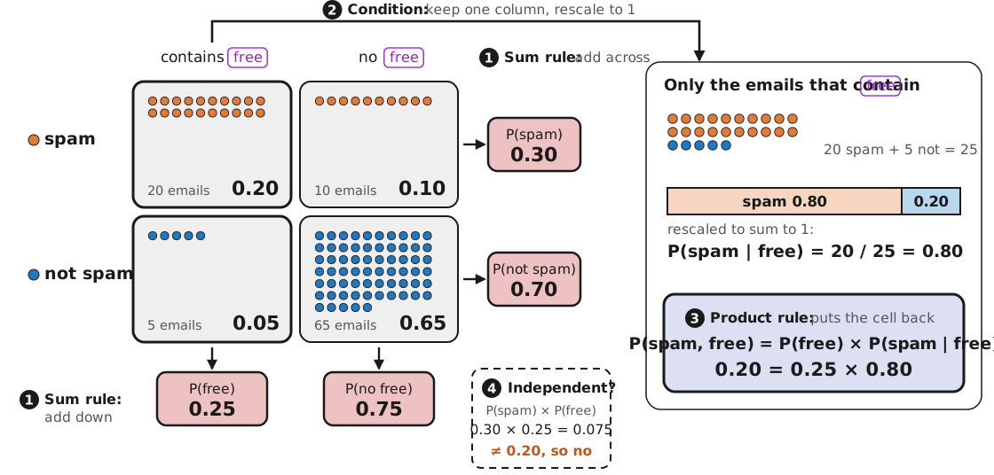
With two values per variable, each move produces a single number. Most inputs a model sees take many values, though, and then the same moves produce whole distributions: each row of the table becomes a histogram, and conditioning gives the shape of one row on its own. To see this, keep \(Y\) as spam or not, let \(X\) be the number of links in an email (0 to 5 or more), and take made-up counts for 200 emails:
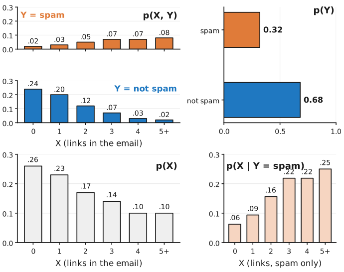
How to read the four panels:
- Top left, the joint \(p(X, Y)\). Each bar is a share of all 200 emails. The first blue bar says that 0.24 of all emails are not spam and have no links; the last orange bar says that 0.08 are spam with five or more links. All twelve bars add up to 1.
- Top right, \(p(Y)\). Add up a row. The six orange bars add up to 0.32, so 32% of emails are spam; the blue bars add up to 0.68.
- Bottom left, \(p(X)\). Add the orange and the blue bar for the same number of links. For no links: \(0.02 + 0.24 = 0.26\).
- Bottom right, \(p(X \mid Y = \text{spam})\). Look at spam only. Divide each orange bar by 0.32 so that the spam bars add up to 1. For five or more links: \(0.08 / 0.32 = 0.25\), so a quarter of spam has five or more links, against about 3% of ordinary email (\(0.02 / 0.68\)).
The bottom-right panel answers “how many links does spam usually have?” A spam filter needs the reverse question: given the links in this email, how likely is it to be spam? Turning one conditional into the other is the job of Bayes’ theorem. Because \(p(X, Y) = p(Y, X)\), applying the product rule both ways and dividing gives it:
\[p(Y \mid X) = \frac{p(X \mid Y)\, p(Y)}{p(X)}, \qquad p(X) = \sum_{Y} p(X \mid Y)\, p(Y).\]In practice we usually know only one direction. A medical test is checked in the lab on people whose condition is already known, so we know \(P(\text{positive} \mid \text{sick})\): how often it catches the disease. But a patient holding a positive result needs the other direction, \(P(\text{sick} \mid \text{positive})\): do I actually have it? Hold on to this reversal. It is the same one at the heart of learning, where the data tell us \(p(\text{data} \mid \theta)\) and we want \(\theta\).
Bayes’ theorem on a medical test
Here is the theorem doing real work. A screening test for a disease is part of a routine checkup. Suppose:
- \(P(\text{sick}) = 0.005\): 0.5% of people have the disease. This is the prior.
- \(P(\text{positive} \mid \text{sick}) = 0.95\): the test is positive for 95% of the people who have it.
- \(P(\text{positive} \mid \text{healthy}) = 0.02\): it is also positive for 2% of healthy people, a false alarm.
Your test comes back positive. How likely is it that you have the disease? Many people answer “about 95%”. Bayes’ theorem says otherwise:
\[P(\text{sick} \mid \text{positive}) = \frac{0.95 \times 0.005}{0.95 \times 0.005 + 0.02 \times 0.995} \approx 0.193.\]Fewer than one positive result in five comes from someone who is sick. The test is good, but healthy people outnumber sick ones 199 to 1, so its small false-alarm rate, applied to that huge pool, produces most of the positives.In counts. Out of 100,000 people, 500 are sick and 475 of them test positive; 99,500 are healthy and 1,990 of them test positive. 475 of 2,465 positives is 19%. That is why a positive screening result is followed by a second, more precise test. We can check the formula by simulating a million people:The forgotten ingredient. A classifier’s output, like this test’s result, becomes a useful probability only once it is combined with how common each class is. A model trained on rebalanced 50/50 data reports probabilities for a 50/50 world.
prior, sens, false_pos = 0.005, 0.95, 0.02

exact = sens * prior / (sens * prior + false_pos * (1 - prior))

n = 1_000_000
is_sick = rng.random(n) < prior
positive = np.where(is_sick, rng.random(n) < sens, rng.random(n) < false_pos)
print(f"Bayes' theorem           : {exact:.4f}")
print(f"simulated, {n:,} people: {is_sick[positive].mean():.4f}"
      f"  ({positive.sum():,} positives, {is_sick[positive].sum():,} of them sick)")
Bayes' theorem           : 0.1927
simulated, 1,000,000 people: 0.1922  (24,402 positives, 4,689 of them sick)
Expectation and variance
A distribution says how likely every value is, which is often more than we need. Two numbers summarize it: where the values typically fall, and how widely they spread.
Expectation: where the values fall. The expectation, or mean, is the average you would get if you drew from the distribution over and over. Weight each value by its probability and add up:
\[\mathbb{E}[t] = \sum_{t} t\, p(t).\]For the coin from the bar chart, 10 tosses with heads probability 0.7, this gives 7 heads, 70% of 10.Not always a possible value. With a heads probability of 0.65 the mean is 6.5, though no run of ten tosses gives six and a half heads.
Variance: how far the values spread. Two distributions can share a mean and still look very different. The variance measures the scatter: take each value’s distance from the mean, square it, and average with the same probability weights:Why square? Misses on either side both count as positive, and big misses count extra.
\[\operatorname{var}[t] = \mathbb{E}\big[(t - \mathbb{E}[t])^2\big] = \sum_{t} (t - \mathbb{E}[t])^2\, p(t).\]For the coin the variance is 2.1, so the standard deviation, its square root, is \(\sqrt{2.1} \approx 1.45\) heads: a typical run of ten lands between 6 and 8 heads.Two different numbers. The 0.7 is about a single toss, which is why ten tosses average 7 heads. The 1.45 is about the whole run: repeat the ten tosses and the count wobbles around 7 by about 1.45 either way. That is the double arrow in the figure below. For a continuous variable the sums become integrals.Continuous case. \(\mathbb{E}[t] = \int t\, p(t)\, dt\), and nothing else changes. The coin in code:For the mathematically inclined. Expectation is linear, \(\mathbb{E}[a t + b u] = a\,\mathbb{E}[t] + b\,\mathbb{E}[u]\), and \(\operatorname{var}[t] = \mathbb{E}[t^2] - \mathbb{E}[t]^2\). For \(N\) tosses these give \(\mathbb{E}[k] = N\theta\) and \(\operatorname{var}[k] = N\theta(1-\theta)\): 7 and 2.1 here.
from math import comb

k = np.arange(11)
p_k = np.array([comb(10, i) * 0.7**i * 0.3**(10 - i) for i in k])
mean = np.sum(k * p_k)
var = np.sum((k - mean) ** 2 * p_k)
print(f"mean = {mean:.2f}, variance = {var:.2f}, standard deviation = {np.sqrt(var):.2f}")
mean = 7.00, variance = 2.10, standard deviation = 1.45
Conditional expectation: the mean for one kind of case. Apply the same averaging to a conditional distribution and you get the conditional expectation \(\mathbb{E}[t \mid \mathbf{x}]\): the average outcome among cases that share the input \(\mathbf{x}\), such as the average sale price of houses with 1,500 square feet. Change \(\mathbf{x}\) and both the center and the spread can move, as the right panel shows.
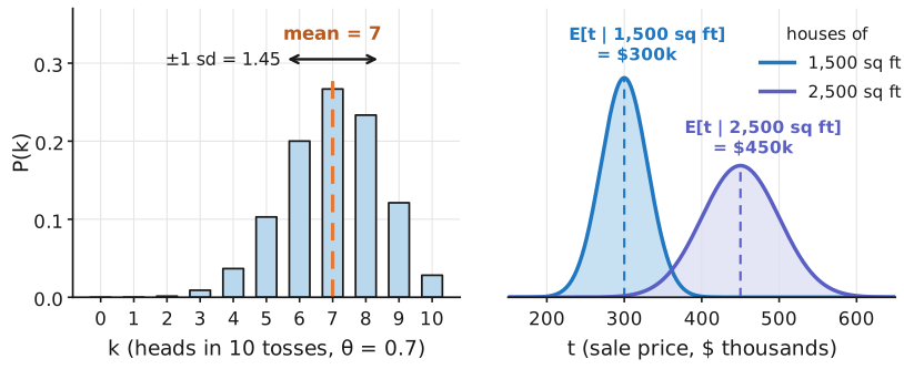
A regression model, seen this way, is trying to learn how \(\mathbb{E}[t \mid \mathbf{x}]\) moves as \(\mathbf{x}\) changes: the line through the centers of all such bells.Coming up. Part 2 (coming soon) shows that training with squared error asks for exactly this quantity.
Likelihood: the same formula, read the other way

Everything so far has assumed that we know the distribution: the coin’s chance of heads, the test’s error rates, the share of spam. Learning runs the other way. We have data, and we need to work out the distribution that produced it. That reversal is step 3 of the pipeline, and the central idea of this post.
Suppose a coin has an unknown probability \(\theta\) of landing heads, and we are given the results of 10 tosses: 7 heads and 3 tails. The question we would really like to answer is “given this data, what is \(\theta\)?”, in symbols \(p(\theta \mid \text{data})\). That question needs a prior, so we start with an easier one.Why it needs a prior. Bayes’ theorem would turn it around, but only with a prior: what we believed about the coin before tossing it, the ingredient the medical-test example showed is easy to get wrong.
The easier question runs the other way, and it works like a thought experiment. Pick a value for \(\theta\), say 0.5, and pretend that is the coin. Toss it 10 times. How likely is it that the ten results come out exactly like the data given to us, the same heads and tails in the same order, say HHTHHHTHHT? A fair coin matches each toss with probability 0.5, so it matches all ten with probability \(0.5^{10} \approx 0.00098\), about once in a thousand tries. For any \(\theta\), each of the 7 heads matches with probability \(\theta\) and each of the 3 tails with probability \(1 - \theta\). The tosses are independent, so the product rule multiplies them:Order matters here. The bar chart earlier asked a looser question: 7 heads in any order. There are 120 such orders, so that probability is 120 times larger, but the factor is the same for every \(\theta\) and changes no comparison.
\[p(\text{data} \mid \theta) = \theta^{7} (1 - \theta)^{3}.\]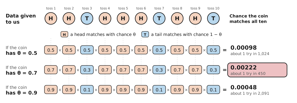
Of the three coins in the figure, \(\theta = 0.7\) explains the data best: it makes our tosses more than twice as probable as a fair coin does.An extreme coin. With \(\theta = 0.1\) the chance is \(0.1^7 \times 0.9^3 \approx 0.00000007\), about 30,000 times smaller than with 0.7.
Read this way, with the data fixed and \(\theta\) the thing we vary, the same expression is called the likelihood:
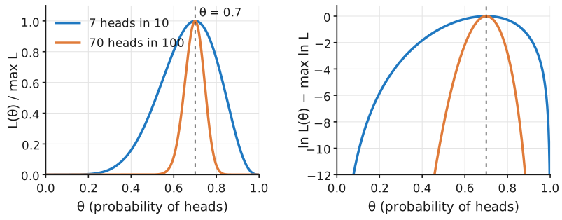
\[L(\theta) = \theta^{7} (1 - \theta)^{3}.\]So one formula has two readings. With \(\theta\) fixed and the data varying, it is a probability. With the data fixed and \(\theta\) varying, it is a likelihood, a score for how well each candidate \(\theta\) explains the data given to us.
The likelihood is not the \(p(\theta \mid \text{data})\) we first wished for. It is not even a probability distribution over \(\theta\): nothing forces it to integrate to 1, and here it does not:
heads, tosses = 7, 10
theta = np.linspace(0, 1, 100_001)
lik = theta**heads * (1 - theta)**(tosses - heads)

print(f"maximizing theta on the grid : {theta[lik.argmax()]:.4f}")
print(f"likelihood at that theta     : {lik.max():.6f}")
print(f"area under L(theta)          : {np.trapezoid(lik, theta):.6f}   (1/1320 = {1/1320:.6f})")
maximizing theta on the grid : 0.7000
likelihood at that theta     : 0.002224
area under L(theta)          : 0.000758   (1/1320 = 0.000758)
The area is \(1/1320\), not 1. For this series we only need the likelihood’s peak.The Bayesian route. Multiplying the likelihood by a prior and rescaling to area 1 gives \(p(\theta \mid \text{data})\). We set that route aside here.
Independence, products, and why we take logs

Step 4 turns the score into something a computer can optimize. The coin’s likelihood had one factor per toss. Real datasets have thousands of observations, and multiplying that many factors causes a practical problem. With \(N\) observations \(t_1, \dots, t_N\) that are independent and identically distributed (i.i.d.),i.i.d. in plain words. Every data point is drawn the same way, and none of them influences another. the product rule with independence makes the likelihood a product of one factor per data point:
\[L(\theta) = \prod_{n=1}^{N} p(t_n \mid \theta).\]Products of many small numbers are unpleasant twice over: their derivatives are messy, and the product quickly falls below the smallest number a computer can represent, so it rounds to exactly zero:How small? A double-precision float bottoms out around \(10^{-308}\). Two thousand Gaussian densities of typical size multiply to about \(10^{-1800}\).
x = rng.normal(loc=3.0, scale=2.0, size=2000)
dens = gauss_pdf(x, 3.0, 2.0)

print(f"product of densities  : {np.prod(dens)}")
print(f"sum of log-densities  : {np.sum(np.log(dens)):.2f}")
print(f"so the likelihood is about 10^{np.sum(np.log(dens)) / np.log(10):.0f}")
product of densities  : 0.0
sum of log-densities  : -4216.49
so the likelihood is about 10^-1831
The fix is to work with the log-likelihood, \(\ln L(\theta) = \sum_n \ln p(t_n \mid \theta)\). The logarithm turns the product into a sum, which is easy to differentiate and has no underflow problem. And because \(\ln\) is strictly increasing, it never moves the maximum: whatever \(\theta\) maximizes \(L\) also maximizes \(\ln L\) (the right panel of the likelihood figure).
The last move is to flip the sign. Optimizers are built to minimize, so we use the negative log-likelihood \(-\ln L(\theta)\), where lower is better. That is the loss in step 4. Maximizing \(\ln L\) and minimizing \(-\ln L\) pick the same \(\theta\), so the next section uses whichever reads more naturally.A deeper reading. \(-\ln p\) is the “surprise” of an outcome: 0 when the model gave it probability 1, large when the model found it unlikely. Training makes the model less surprised by the data.
Maximum likelihood

We now have the pieces for step 5, training: find the parameter value with the lowest loss, which is the same as the highest likelihood. The maximum likelihood estimate (MLE) is the parameter value that maximizes the likelihood, or equivalently the log-likelihood:
\[\theta_{\text{ML}} = \arg\max_{\theta} \sum_{n=1}^{N} \ln p(t_n \mid \theta).\]For the coin we can find it with calculus. With \(k\) heads in \(N\) tosses the log-likelihood is \(k \ln \theta + (N - k) \ln (1 - \theta)\). Setting its derivative to zero,
\[\frac{k}{\theta} - \frac{N - k}{1 - \theta} = 0 \quad\Longrightarrow\quad \theta_{\text{ML}} = \frac{k}{N},\]the fraction of heads, which is what intuition suggests and what the grid search found.The steps. The derivative of \(k \ln \theta\) is \(k/\theta\), and of \((N-k)\ln(1-\theta)\) it is \(-(N-k)/(1-\theta)\). Setting their sum to zero gives \(k(1-\theta) = (N-k)\theta\), so \(\theta = k/N\).
The Gaussian case
The distribution that matters most for this series is the Gaussian, or normal distribution: the bell curve. For a real number \(t\) with mean \(\mu\) and variance \(\sigma^2\), its density is
\[\mathcal{N}(t \mid \mu, \sigma^2) = \frac{1}{\sqrt{2\pi\sigma^2}} \exp\!\left( -\frac{(t - \mu)^2}{2\sigma^2} \right).\]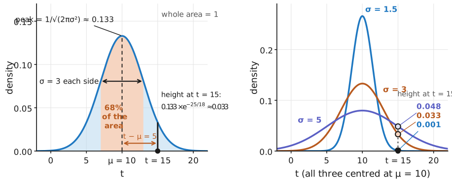
Read the formula from the inside out, following the left panel, where \(\mu = 10\), \(\sigma = 3\), and one point sits at \(t = 15\). \((t - \mu)^2\) is the squared distance from the center, here \(5^2 = 25\). Dividing by \(2\sigma^2 = 18\) measures that distance against the spread. The exponential of minus that number is 1 at the center and falls away quickly on both sides, which gives the bell its shape; at \(t = 15\) it is \(e^{-25/18} \approx 0.25\). The constant in front only scales the curve so that the total area is 1. Here it sets the peak at \(1/\sqrt{2\pi \cdot 9} \approx 0.133\), so the height at \(t = 15\) is \(0.133 \times 0.25 \approx 0.033\). The right panel shows what \(\sigma\) does: a wide bell is lower at its peak but forgives a far-off point more than a narrow one does.The earlier bell. With \(\sigma = 0.1\) the same constant gives the peak \(1/(0.1\sqrt{2\pi}) \approx 3.99\), the number the code printed.
Why this curve, out of every possible bump? Mainly because it shows up in real data. When a quantity is the sum of many small, independent effects, like the unrecorded kitchens, buyers, and timing that nudge a house price, the total tends toward a Gaussian whatever the individual effects look like. That is the central limit theorem.Two more reasons. Among all distributions with a given mean and variance, the Gaussian assumes the least (it has the largest entropy). And its logarithm is a plain quadratic, as we are about to see.
Now run it through the pipeline. For \(N\) i.i.d. points the likelihood is a product of one Gaussian per point (step 3), and the logarithm turns it into a sum (step 4):
\[\ln L(\mu, \sigma^2) = \sum_{n=1}^{N} \ln \mathcal{N}(t_n \mid \mu, \sigma^2).\]Take one term at a time. The log of a product is the sum of the logs, and the log undoes the exponential:
\[\begin{aligned} \ln \mathcal{N}(t_n \mid \mu, \sigma^2) &= \ln \frac{1}{\sqrt{2\pi\sigma^2}} + \ln \exp\!\left( -\frac{(t_n - \mu)^2}{2\sigma^2} \right) \\ &= -\tfrac{1}{2} \ln(2\pi\sigma^2) - \frac{(t_n - \mu)^2}{2\sigma^2} \\ &= -\frac{(t_n - \mu)^2}{2\sigma^2} - \tfrac{1}{2} \ln \sigma^2 - \tfrac{1}{2} \ln(2\pi). \end{aligned}\]The second line uses \(\ln(1/\sqrt{a}) = -\tfrac{1}{2} \ln a\), and the third splits \(\ln(2\pi\sigma^2)\) into \(\ln \sigma^2 + \ln(2\pi)\). Adding up the \(N\) terms, the last two pieces are the same for every point, so they are simply counted \(N\) times:
\[\ln L(\mu, \sigma^2) = -\frac{1}{2\sigma^2} \sum_{n=1}^{N} (t_n - \mu)^2 - \frac{N}{2} \ln \sigma^2 - \frac{N}{2} \ln(2\pi).\]Look at how \(\mu\) enters: only through the sum of squared differences \(\sum_n (t_n - \mu)^2\), multiplied by a negative constant. Maximizing the likelihood over \(\mu\) is therefore the same as minimizing a sum of squares. That single observation is the heart of Part 2. The figure shows it on eight points.
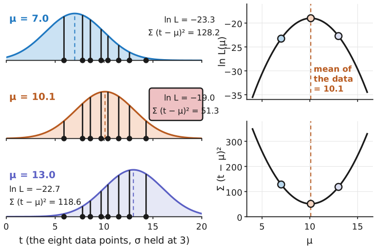
To find the best \(\mu\) (step 5), set the derivative to zero. Only the first term contains \(\mu\), and the derivative of \((t_n - \mu)^2\) with respect to \(\mu\) is \(-2(t_n - \mu)\), so
\[\frac{\partial \ln L}{\partial \mu} = \frac{1}{\sigma^2} \sum_{n=1}^{N} (t_n - \mu) = 0 \quad\Longrightarrow\quad \sum_{n=1}^{N} t_n = N\mu \quad\Longrightarrow\quad \mu_{\text{ML}} = \frac{1}{N} \sum_{n=1}^{N} t_n.\]The same move with respect to \(\sigma^2\) (exercise 5 walks through it) gives
\[\sigma^2_{\text{ML}} = \frac{1}{N} \sum_{n=1}^{N} (t_n - \mu_{\text{ML}})^2:\]the sample mean, and the average squared deviation from it.Watch out with little data. Three tosses, three heads: the MLE is \(\theta = 1\), a coin that never lands tails. The Gaussian \(\sigma^2_{\text{ML}}\) divides by \(N\) and comes out too small on average, which is why the sample variance divides by \(N - 1\). Priors and regularization fix this; see the end of Part 2. To check the algebra, compare the formulas with a general-purpose optimizer that knows nothing about them:Why ln σ? Optimizing \(\ln \sigma\) rather than \(\sigma\) keeps the optimizer from stepping to a negative standard deviation.
def neg_log_lik(params, t):
    mu, log_sigma = params
    sigma = np.exp(log_sigma)
    return 0.5 * np.sum(((t - mu) / sigma) ** 2) + len(t) * log_sigma + 0.5 * len(t) * np.log(2 * np.pi)

t = rng.normal(loc=10.0, scale=3.0, size=200)
res = minimize(neg_log_lik, x0=[0.0, 0.0], args=(t,))

print(f"closed form : mu = {t.mean():.4f}, sigma^2 = {np.mean((t - t.mean())**2):.4f}")
print(f"optimizer   : mu = {res.x[0]:.4f}, sigma^2 = {np.exp(2 * res.x[1]):.4f}")
closed form : mu = 10.3282, sigma^2 = 11.0796
optimizer   : mu = 10.3282, sigma^2 = 11.0796
From likelihood to loss
We have now walked steps 1 to 5 with a coin. So far the parameters described one distribution for all the data. A predictive model makes the distribution depend on the input: the network or regression function with weights \(\mathbf{w}\) maps \(\mathbf{x}\) to the parameters of \(p(t \mid \mathbf{x}, \mathbf{w})\), for example the mean of a Gaussian or the probability of a coin. Given training pairs \((\mathbf{x}_n, t_n)\), the log-likelihood of the weights is
\[\ln L(\mathbf{w}) = \sum_{n=1}^{N} \ln p(t_n \mid \mathbf{x}_n, \mathbf{w}).\]As in step 4, we flip the sign, and we usually divide by \(N\). The result is the negative log-likelihood (NLL), and it is the loss:
Result. For any probability model \(p(t \mid \mathbf{x}, \mathbf{w})\), maximum likelihood training means minimizing
\[E(\mathbf{w}) = -\frac{1}{N} \sum_{n=1}^{N} \ln p(t_n \mid \mathbf{x}_n, \mathbf{w}).\]Choose the distribution, and the loss follows. Gradient descent then does the minimizing.
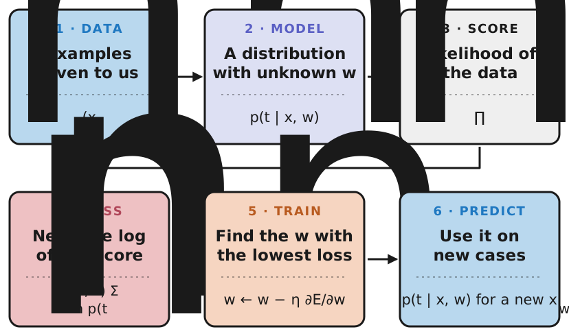
Every common loss comes from one choice in step 2:
| What the target is | Distribution assumed for \(t\) given \(\mathbf{x}\) | Negative log-likelihood (the loss) | Covered in |
|---|---|---|---|
| a real number | Gaussian with mean \(y(\mathbf{x}, \mathbf{w})\) | squared error | Part 2 |
| a real number, with outliers | Laplace with location \(y(\mathbf{x}, \mathbf{w})\) | absolute error | Part 2 |
| one of two labels | Bernoulli with probability \(y(\mathbf{x}, \mathbf{w})\) | binary cross-entropy | Part 3 |
| one of \(K\) labels | categorical with probabilities \(y_k(\mathbf{x}, \mathbf{w})\) | cross-entropy | Part 3 |
| a count (0, 1, 2, …) | Poisson with rate \(y(\mathbf{x}, \mathbf{w})\) | Poisson deviance | exercise 7 |
That table is the whole series in miniature.Coming up. Part 2 (coming soon) takes the first two rows: squared error from Gaussian noise, and what to do when the noise is not Gaussian. Part 3 (coming soon) takes the label rows: why cross-entropy, not squared error, is the loss for classification.
Summary
- A predictive model is best understood as a conditional distribution \(p(t \mid \mathbf{x}, \mathbf{w})\); a point prediction is one summary of it.
- The sum and product rules give Bayes’ theorem. Base rates matter: when a disease affects 0.5% of people, a test that catches 95% of cases with a 2% false-alarm rate is right less than one time in five when it says positive.
- The likelihood is the probability of the observed data, read as a function of the parameters. It is not a distribution over the parameters.
- We maximize the log-likelihood instead of the likelihood: same maximizer, sums instead of products, no underflow.
- Maximum likelihood for a Gaussian mean is least squares. Maximum likelihood for a predictive model is minimizing the negative log-likelihood, and that NLL is the loss function.
Exercises
- For the bar chart of heads in 10 tosses, show by counting coin-toss sequences that the probability of \(k\) heads in 10 tosses is \(P(k) = \binom{10}{k}\theta^{k}(1-\theta)^{10-k}\). With \(\theta = 0.7\), compute \(P(7)\) and \(P(k \ge 8)\) by hand, and use the binomial theorem to show that the eleven bars sum to 1.
- For the bell curve beside it, compute the peak height \(p(0)\) from the Gaussian formula with \(\sigma = 0.1\). Show numerically that \(P(-0.1 \le t \le 0.1) \approx 0.683\). Then compare \(P(-0.005 \le t \le 0.005)\) with \(p(0) \times 0.01\), and explain in what sense a density is “probability per unit length”.
- Repeat the medical-test calculation with a false-alarm rate of 0.5% instead of 2%. What fraction of positive results are sick now? Which change helps more: cutting the false-alarm rate from 2% to 1%, or raising the sensitivity from 95% to 99%?
- Show that the area under \(L(\theta) = \theta^{k}(1 - \theta)^{N - k}\) on \([0, 1]\) is \(\frac{k!\,(N - k)!}{(N + 1)!}\), and check it for \(k = 7\), \(N = 10\). (Hint: the Beta function.)
- Derive \(\sigma^2_{\text{ML}}\) for the Gaussian by setting the derivative of the log-likelihood with respect to \(\sigma^2\) to zero. (Hint: write \(s = \sigma^2\) and differentiate \(-\frac{1}{2s} \sum_n (t_n - \mu)^2 - \frac{N}{2} \ln s\) with respect to \(s\).) Then show by simulation that \(\mathbb{E}[\sigma^2_{\text{ML}}] = \frac{N - 1}{N} \sigma^2\): draw many samples of size \(N = 5\) and average the estimates.
- The underflow cell used 2000 points. Find, by experiment, roughly how many points it takes before
np.prod(dens)returns exactly zero for that Gaussian. - A Poisson distribution for counts has \(p(t \mid \lambda) = \lambda^{t} e^{-\lambda} / t!\). Write the negative log-likelihood for a model that predicts \(\lambda = \exp(\mathbf{w}^{\mathrm{T}} \mathbf{x})\), and drop the terms that do not depend on \(\mathbf{w}\). This is the loss for count regression.
- In your own words: why is “the likelihood of \(\theta\)” not “the probability of \(\theta\)”? What extra ingredient would turn one into the other?
Going further
- The CSE 474/574 notes develop all of this at course depth: Intro to ML, module 01 covers the probability rules, Gaussian maximum likelihood and its bias, and least squares as maximum likelihood; module 02 covers the standard distributions and Bayesian estimation with priors.
- The CSE 676 notes revisit the same ground from the deep learning side in Deep Learning, module 02.
- C. M. Bishop, Pattern Recognition and Machine Learning (2006), chapters 1 and 2, freely available as a PDF.
- D. J. C. MacKay, Information Theory, Inference, and Learning Algorithms (2003), free to read online; chapters 2 and 3 are an unusually clear introduction to probability and inference.
Questions, corrections, or a topic you would like me to write about? Write to me. New pieces are announced in the feed.